8 But side effects that are ignored?

(where you learn why the market fails to save the environment)

Markets are not always the flawless mechanism that ensures goods and services are produced in socially optimal quantities. In the previous chapter I showed that markets can fail when one actor gains excessive power — for example in monopoly and monopsony. But there are other market failures. The picture below shows what I encountered at the Market Square on a Sunday morning in August:

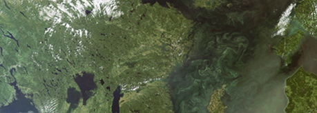
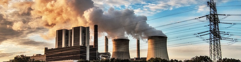
It looks like Finns had a merry Saturday night — perhaps a little too merry. These nuisance effects of alcohol consumption are examples of negative externalities. An externality occurs when a transaction between a buyer and a seller affects a third party: when you (the buyer) buy booze from Alko (the seller) it also affects me (the third party). If you only think about your own interests and ignore that your drinking causes unpleasant side effects that cloud my life, you will consume more alcohol than is socially desirable. In other words: externalities cause markets to fail. The same mechanism that explains the litter at the Market Square can account for many other environmental problems on the planet. Understanding externalities therefore not only makes you see why the problems arise, it also clarifies what politicians and policymakers must actually do to, for example, tackle Baltic Sea eutrophication or global warming. That is the purpose of this chapter.

8.1 Externalities

There are many situations where an exchange between two parties also affects people who are not directly involved. In the table below I have listed some examples:

Negative externalities	Positive externalities
alcohol abuse	education
smoking	vaccination
overuse of antibiotics	perfume (scent)
industrial air pollution	a beautiful garden
neighbors causing disturbances	beehives near farmland
traffic congestion	scientific discoveries
overfishing	street art
your own example?	your own example?

Table 8.1: Examples of externalities. Can you think of your own example?

Smoking is a classic example of a negative externality. Preferences, prices and incomes determine how many cigarettes you choose to buy, as we saw in Chapter 6. But if your smoking also harms people around you — think passive smoking — and you ignore these side effects when deciding how much to smoke, then you will smoke excessively. Or imagine you weigh your own pros and cons and decide to take antibiotics every time you catch a cold. It is likely you have forgotten to account for the fact that your consumption also contributes to the development of resistant bacteria, which makes antibiotics ineffective in the future and can cause people to die.

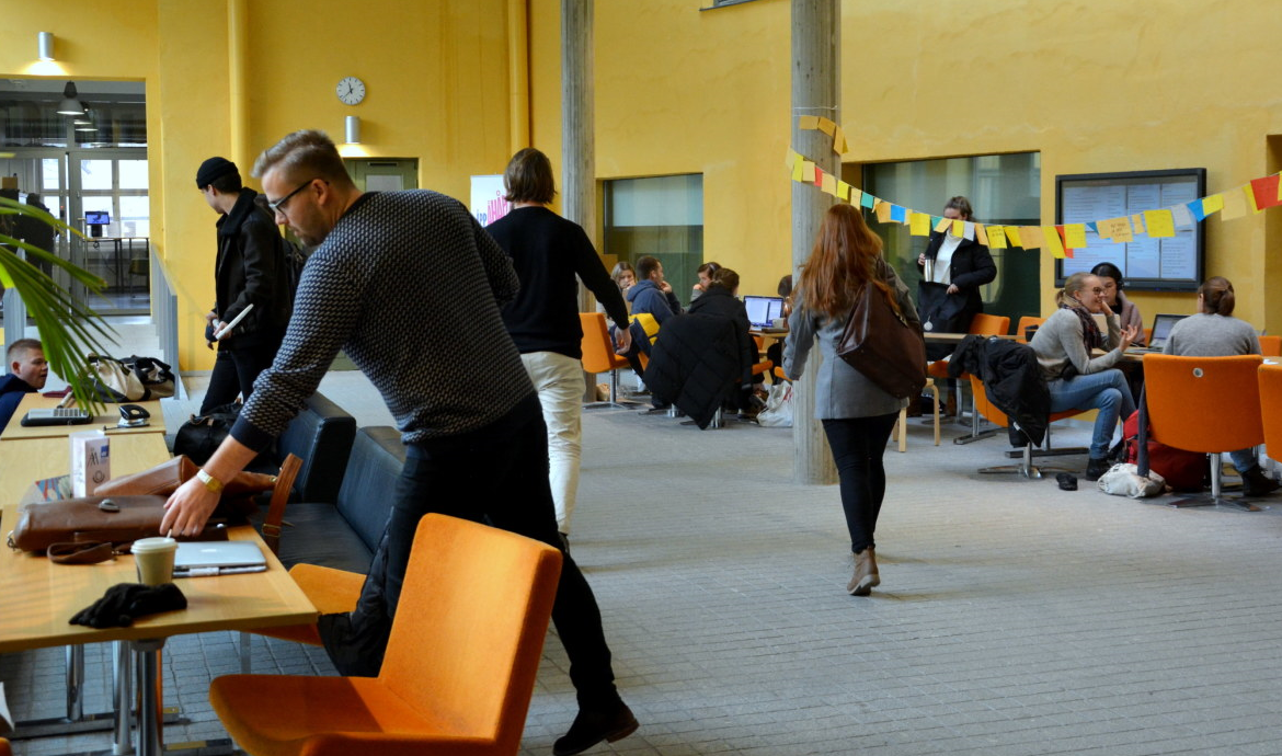
Similarly there are situations where an interaction between two parties benefits others — so‑called positive externalities. Education is an example: getting a higher education helps not only you but also those around you. For instance, you will probably train your future colleagues at work. It’s almost as if they’re invisibly sitting on a chair next to you right now. Some even argue that higher education deepens democratic understanding and thus benefits the whole population. Positive externalities therefore also cause market failure. Recall Ronja in Chapter 1 weighing whether to accept a place at Harvard. The private cost was tuition of €120,000 plus the €72,000 she would forgo working at Prisma — a total opportunity cost of €192,000. Do you really think Ronja will account for the fact that her Harvard degree also benefits her future coworkers and democracy in Finland?

In the right‑hand column of Table 8.1 above I listed more examples of positive externalities. For example, vaccinating yourself against COVID‑19 is not only good for you but also for the people around you. Do you understand my other examples in the table — and can you think of even better ones?

8.2 The effects of externalities

We will now examine in detail how markets are affected by externalities. Let’s take the market for e‑scooters as an example. To keep things simple we assume perfect competition, that the market price is €4.50 to rent a scooter for 15 minutes, and that 1,000 such trips are sold each day in Turku. According to our theory 1,000 is the efficient level. How do we know that? Think like this: for most of the trips sold consumers valued the service at more than €4.50 and firms’ costs of providing those trips were below €4.50. But the very last trip sold — the marginal trip — cost exactly €4.50 to produce and was valued by the consumer at exactly €4.50. That means one more trip — number 1,001 — would cost more for firms to provide than a potential customer would value it. Conversely, producing fewer than 1,000 trips would be absurd because there would be consumers out there who value additional trips more than it would cost firms to provide them.

In practice there is, however, a problem: on the left of the figure below you can see an unpleasant side‑effect of e‑scooter trading:

Figure 8.1: **Market and negative externalities.** E‑scooters on a street in Stockholm. Emissions from a factory. A production line where ten live chicks are being ground per second.

Some users apparently throw their e‑scooters onto the street after a ride, which harms the elderly and visually impaired. What happens in the e‑scooter market therefore affects not only riders and rental firms but also bystanders.

»Each e‑scooter trip imposes a €2 cost on the elderly and visually impaired in the form of accidents!« cry the advocacy groups.

Do you see what should happen to scooter rentals if consumers actually took into account that their behaviour imposes a €2 negative externality on the elderly and visually impaired? The intuitive answer is that fewer scooters should be rented, and to achieve this the price must be raised. The app below illustrates this. Can you use the app to determine how many trips would be socially optimal if the advocacy groups are correct that each trip causes a €2 negative externality?

Externalities.
Play with the curves to understand why the market can produce a socially suboptimal outcome when side effects are ignored.

#| standalone: true
#| viewerHeight: 1350

if (!requireNamespace("shiny", quietly = TRUE)) install.packages("shiny")
if (!requireNamespace("ggplot2", quietly = TRUE)) install.packages("ggplot2")
if (!requireNamespace("plotly", quietly = TRUE)) install.packages("plotly")
if (!requireNamespace("grid", quietly = TRUE)) install.packages("grid")

library(shiny)
library(ggplot2)
library(plotly)
library(grid)

safe_numeric <- function(value) {
  if (is.null(value) || value == "" || is.na(value)) return(0)
  as.numeric(value)
}

ui <- fluidPage(
  fluidRow(
    column(4,
           wellPanel(
             numericInput("supply_intercept", "Ange interceptet för utbudskurvan:", 2.5),
             numericInput("supply_slope", "Ange lutningen för utbudskurvan (positiv):", 0.002, min = 1e-6),
             numericInput("demand_intercept", "Ange interceptet för efterfrågekurvan:", 10.5),
             numericInput("demand_slope", "Ange lutningen för efterfrågekurvan (negativ):", -0.006, max = -1e-6),
             numericInput("externality", "Ange externaliteten (OBS! Negativt tal för negativa externaliteter):", 0, step = 0.25),
             numericInput("x_max", "X-axelns maxvärde i figuren:", value = 2000, min = 1),
             numericInput("y_max", "Y-axelns maxvärde i figuren:", value = 15, min = 1),
             actionButton("update", "Uppdatera figuren och beräkningarna",
                          style = "color: white; background-color: #007bff; padding: 6px 12px; border: 2px solid #007bff; font-size: 14px;"),
             br(),
             tags$h5("OBS! Ange ett NEGATIVT tal om du har en negativ externalitet (t.ex. -5). Ange ett POSITIVT tal om du har en positiv externalitet (t.ex. 5): Klicka på 'Uppdatera figuren och beräkningarna'."),
             tags$small("Obs: Utbudskurvan måste ha positiv lutning och efterfrågekurvan negativ.")
           )
    ),
    column(8,
           plotlyOutput("demandSupplyPlot"),
           br(),
           verbatimTextOutput("equilibrium"),
           verbatimTextOutput("optimalProduction"),
           verbatimTextOutput("inverseFunctions")
    )
  )
)

server <- function(input, output, session) {
  validatedInput <- reactiveValues(
    supply_intercept = 2.5,
    supply_slope = 0.002,
    demand_intercept = 10.5,
    demand_slope = -0.006,
    externality = 0,
    x_max = 2000,
    y_max = 15
  )

  observeEvent(input$update, {
    # basic validation and store
    si <- safe_numeric(input$supply_intercept)
    ss <- safe_numeric(input$supply_slope)
    di <- safe_numeric(input$demand_intercept)
    ds <- safe_numeric(input$demand_slope)
    ext <- safe_numeric(input$externality)
    xm <- max(1, safe_numeric(input$x_max))
    ym <- max(1, safe_numeric(input$y_max))

    if (ss <= 0) {
      showNotification("Utbudslutningen måste vara ett positivt tal.", type = "error")
      return()
    }
    if (ds >= 0) {
      showNotification("Efterfrågelutningen måste vara ett negativt tal.", type = "error")
      return()
    }

    validatedInput$supply_intercept <- si
    validatedInput$supply_slope     <- ss
    validatedInput$demand_intercept <- di
    validatedInput$demand_slope     <- ds
    validatedInput$externality      <- ext
    validatedInput$x_max            <- xm
    validatedInput$y_max            <- ym

    showNotification("Parametrar uppdaterade.", type = "message")
  })

  equilibrium <- reactive({
    si <- validatedInput$supply_intercept
    ss <- validatedInput$supply_slope
    di <- validatedInput$demand_intercept
    ds <- validatedInput$demand_slope

    if (abs(ss - ds) < .Machine$double.eps^0.5) return(list(eq_x = NA, eq_y = NA))
    eq_x <- (di - si) / (ss - ds)
    eq_y <- si + ss * eq_x
    if (is.na(eq_x) || is.na(eq_y) || eq_x < 0 || eq_y < 0) return(list(eq_x = NA, eq_y = NA))
    list(eq_x = eq_x, eq_y = eq_y)
  })

  optimal <- reactive({
    si <- validatedInput$supply_intercept
    ss <- validatedInput$supply_slope
    di <- validatedInput$demand_intercept
    ds <- validatedInput$demand_slope
    ext <- validatedInput$externality

    # Positive externality -> demand shifts up by ext
    # Negative externality -> supply shifts up by |ext| (external cost)
    if (ext > 0) {
      adj_di <- di + ext
      opt_x <- (adj_di - si) / (ss - ds)
      opt_y <- si + ss * opt_x
    } else {
      adj_si <- si + abs(ext)
      opt_x <- (di - adj_si) / (ss - ds)
      opt_y <- adj_si + ss * opt_x
    }

    if (is.na(opt_x) || is.na(opt_y) || opt_x < 0 || opt_y < 0) return(list(opt_x = NA, opt_y = NA))
    list(opt_x = opt_x, opt_y = opt_y)
  })

  output$equilibrium <- renderText({
    eq <- equilibrium()
    if (is.na(eq$eq_x)) {
      "Jämvikt: Ingen skärningspunkt vid positiva värden"
    } else {
      paste0("Marknadsjämvikt:\nPris: ", round(eq$eq_y, 3), "\nMängd: ", round(eq$eq_x, 3))
    }
  })

  output$optimalProduction <- renderText({
    opt <- optimal()
    if (is.na(opt$opt_x)) {
      "Samhällsoptimal produktion: Ingen skärningspunkt vid positiva värden"
    } else {
      paste0("Samhällsoptimal produktion (med externalitet):\nPris: ", round(opt$opt_y, 3), "\nMängd: ", round(opt$opt_x, 3))
    }
  })

  output$demandSupplyPlot <- renderPlotly({
    si <- validatedInput$supply_intercept
    ss <- validatedInput$supply_slope
    di <- validatedInput$demand_intercept
    ds <- validatedInput$demand_slope
    ext <- validatedInput$externality
    x_max <- validatedInput$x_max
    y_max <- validatedInput$y_max

    q <- seq(0, x_max, length.out = 400)
    y_supply <- si + ss * q
    y_demand <- di + ds * q

    if (ext > 0) {
      y_opt_demand <- (di + ext) + ds * q
      y_opt_supply <- y_supply
      opt_label_color <- "green"
    } else if (ext < 0) {
      y_opt_supply <- (si + abs(ext)) + ss * q
      y_opt_demand <- y_demand
      opt_label_color <- "orange"
    } else {
      y_opt_supply <- y_supply
      y_opt_demand <- y_demand
      opt_label_color <- "grey30"
    }

    data <- data.frame(q = q,
                       Supply = y_supply,
                       Demand = y_demand,
                       OptimalSupply = y_opt_supply,
                       OptimalDemand = y_opt_demand)

    # Keep rows where at least one curve is >= 0 (so markers are visible)
    data <- data[ (data$Supply >= 0) | (data$Demand >= 0) | (data$OptimalSupply >= 0) | (data$OptimalDemand >= 0), ]

    eq <- equilibrium()
    opt <- optimal()

    p <- ggplot(data, aes(x = q)) +
      geom_line(aes(y = Supply, color = "Utbud"), size = 1) +
      geom_line(aes(y = Demand, color = "Efterfrågan"), size = 1) +
      geom_line(aes(y = OptimalSupply, color = "'Optimalt' utbud"), linetype = "dotted", size = 1) +
      geom_line(aes(y = OptimalDemand, color = "'Optimal' efterfrågan"), linetype = "dotted", size = 1) +
      labs(x = "Mängd (Q)", y = "Pris (P)", color = NULL) +
      coord_cartesian(xlim = c(0, x_max), ylim = c(0, y_max)) +
      scale_color_manual(
        values = c("Utbud" = "#1b9e77", "Efterfrågan" = "#d95f02",
                   "'Optimal' efterfrågan" = "#377eb8", "'Optimalt' utbud" = "#ffa500"),
        guide = guide_legend(override.aes = list(size = 0.9,
                                                 linetype = c("solid", "solid", "dotted", "dotted")))
      ) +
      theme_minimal(base_size = 14) +
      theme(
        axis.title = element_text(size = 14, face = "bold"),
        axis.text = element_text(size = 12),
        legend.position = c(0.90, 0.85),
        legend.background = element_rect(fill = "white", color = "grey80", size = 0.5),
        legend.key = element_rect(fill = "transparent", color = NA),
        legend.text = element_text(size = 11),
        plot.margin = margin(10, 10, 10, 10)
      ) +
      geom_hline(yintercept = 0, color = "black", size = 0.6) +
      geom_vline(xintercept = 0, color = "black", size = 0.6)

    # Mark equilibrium and social optimum if valid
    if (!is.na(eq$eq_x)) {
      p <- p +
        geom_point(aes(x = eq$eq_x, y = eq$eq_y), color = "purple", size = 3) +
        geom_segment(aes(x = eq$eq_x, xend = eq$eq_x, y = 0, yend = eq$eq_y), linetype = "dashed", color = "purple") +
        geom_segment(aes(x = 0, xend = eq$eq_x, y = eq$eq_y, yend = eq$eq_y), linetype = "dashed", color = "purple")
    }

    if (!is.na(opt$opt_x)) {
      p <- p +
        geom_point(aes(x = opt$opt_x, y = opt$opt_y), color = opt_label_color, size = 3) +
        geom_segment(aes(x = opt$opt_x, xend = opt$opt_x, y = 0, yend = opt$opt_y), linetype = "dashed", color = opt_label_color) +
        geom_segment(aes(x = 0, xend = opt$opt_x, y = opt$opt_y, yend = opt$opt_y), linetype = "dashed", color = opt_label_color)
    }

    ggplotly(p) %>%
      layout(
        font = list(size = 13, family = "Arial"),
        legend = list(bgcolor = "rgba(255,255,255,0.95)", x = 0.92, y = 0.85, xanchor = "right",
                      font = list(size = 11)),
        margin = list(l = 60, r = 60, t = 10, b = 60)
      )
  })

  output$inverseFunctions <- renderText({
    si <- validatedInput$supply_intercept
    ss <- validatedInput$supply_slope
    di <- validatedInput$demand_intercept
    ds <- validatedInput$demand_slope

    supply_inverse <- if (ss != 0) {
      paste0("Q = (P - ", si, ") / ", ss)
    } else "Utbudslinjen kan inte inverteras (lutning = 0)."

    demand_inverse <- if (ds != 0) {
      paste0("Q = (P - ", di, ") / ", ds)
    } else "Efterfrågelinjen kan inte inverteras (lutning = 0)."

    paste("Utbud: ", supply_inverse, "\nEfterfrågan: ", demand_inverse)
  })
}

shinyApp(ui = ui, server = server)

Think of it this way to understand the app: in the baseline the supply curve is $\small P_S=2.5+0.002Q$ and the demand curve is $\small P_D=10.5-0.006Q$. These market forces imply an equilibrium price of €4.50 and at that price consumers want to buy 1,000 trips.

Make sure: 1) Can you rearrange the expressions to obtain supply $\small Q_S=-1{,}250+500P$ and demand $\small Q_D=1{,}750-166.7P$, 2) Can you draw these curves by hand? If you can’t, look up how to do it and learn this before you continue.

Your intuition should tell you that this market equilibrium results in too many trips. Each trip imposes a nuisance on the elderly and visually impaired, just as your drinking on the square spoiled my Sunday walk. To find the socially optimal number of trips you must include the negative externality in your calculations. According to the advocacy groups the external cost is €2 per trip. Now use the menu at the “Enter externality” field to input “-2” and then click the blue button to update the analysis. The computer will now display a new curve, which I’ve labelled the “Optimal” supply curve. This “supply curve” captures both the firms’ costs AND the costs imposed on third parties. In other words it shows how the supply curve would look if firms were required to account for all costs their activity generates. This curve therefore lies €2 above the original supply curve, which did not account for the negative side effects. Since the original supply curve was $\small P_S=2.5+0.002Q$ the new one must be $\small P_S=4.5+0.002Q$.

You can now compute the socially optimal output by solving 4.5 + 0.002Q = 10.5 − 0.006Q for Q. Can you verify that Q should be 750?

Look again at the figure and make sure you understand why 1,000 trips is not socially optimal. The person who rents the 1,000th trip values it at €4.50, but the total cost of that trip is €6.50 (that is, €4.50 private cost to the firm plus €2 in harm to the elderly and visually impaired). The problem is that firms such as Voi, Tier and Ryde have no incentive to account for these negative side effects, which leads to traffic levels higher (1,000 trips) than the socially optimal level (750). In other words the market fails: we get too much of activities that cause negative externalities and too little of activities that generate positive externalities.

8.3 How to solve environmental problems?

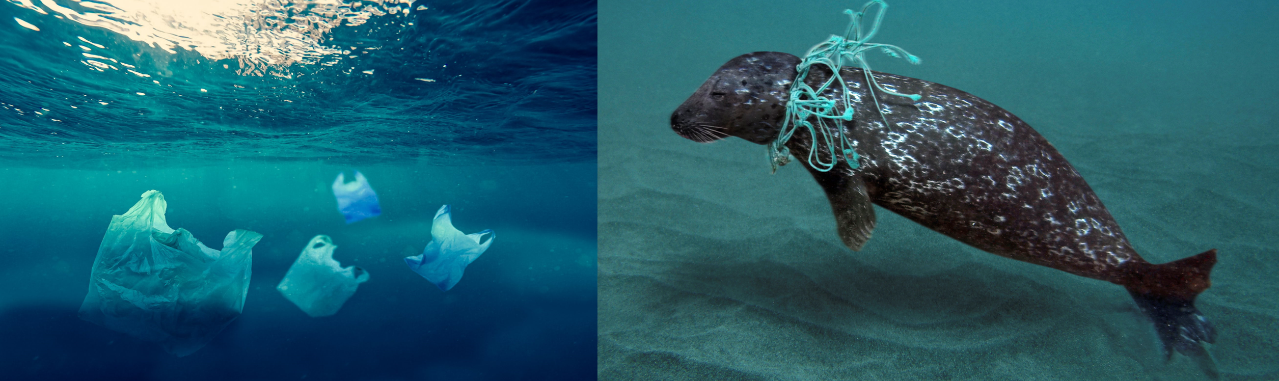
Trade brings huge benefits to the parties on the market. We see this, for example, in consumer and producer surplus. But production can also generate negative externalities. If you sell drugs for children with cancer (good!), there is a risk the packaging will end up in the sea and harm wildlife (bad!). The core problem is that you can often ignore these side effects — they are costs you do not have to bear yourself. So how can we best solve the world’s environmental problems? This is a question you can study in much greater depth on an environmental economics course. In the chapter Mer nationalekonomi? you can read more about the entire economics programme and what each course covers. However, we can already discuss the intuition behind environmental economics here:

Bans and quotas

One first thought might be to ban all activities that generate negative externalities. But reasoning so rigidly often leads you astray. The optimal quantity of something is rarely zero; for example, it would be foolish to ban childhood cancer medicines simply because their packaging sometimes ends up in the sea. In the e‑scooter case in Turku, where the negative externality was €2 per trip, the socially optimal quantity was not zero but 750 trips. Only when each trip imposes a negative externality of €8 or more would a complete ban be optimal.

An alternative is to introduce a quota of 750 trips, as described in Section 5.1. Even though a quota limits trade (which in that case is exactly what we wanted), it can also create challenges. Imagine demand for e‑scooters suddenly rises—perhaps because people increasingly prefer low‑carbon transport or because car taxes are raised. The socially optimal number of e‑scooter trips would then increase (try raising demand in the app yourself!), and the regulator would have to raise the quota quickly. Because market forces constantly change, it will be hopelessly difficult for a bureaucrat to continuously steer the market to the right quantity.

Environmental taxes

A smarter way to think is to change incentives. The core problem is that firms do not have to “take into account” that each trip imposes an extra €2 cost. So how can we force firms to also internalise this effect on third parties? By making firms pay a tax equal to the negative externality. The basic idea is simple: it must hurt the wallet of the polluter. If Voi, Tier and Ryde must pay an extra €2 fee every time they rent a scooter, the firms themselves will then produce the quantity that is socially optimal.

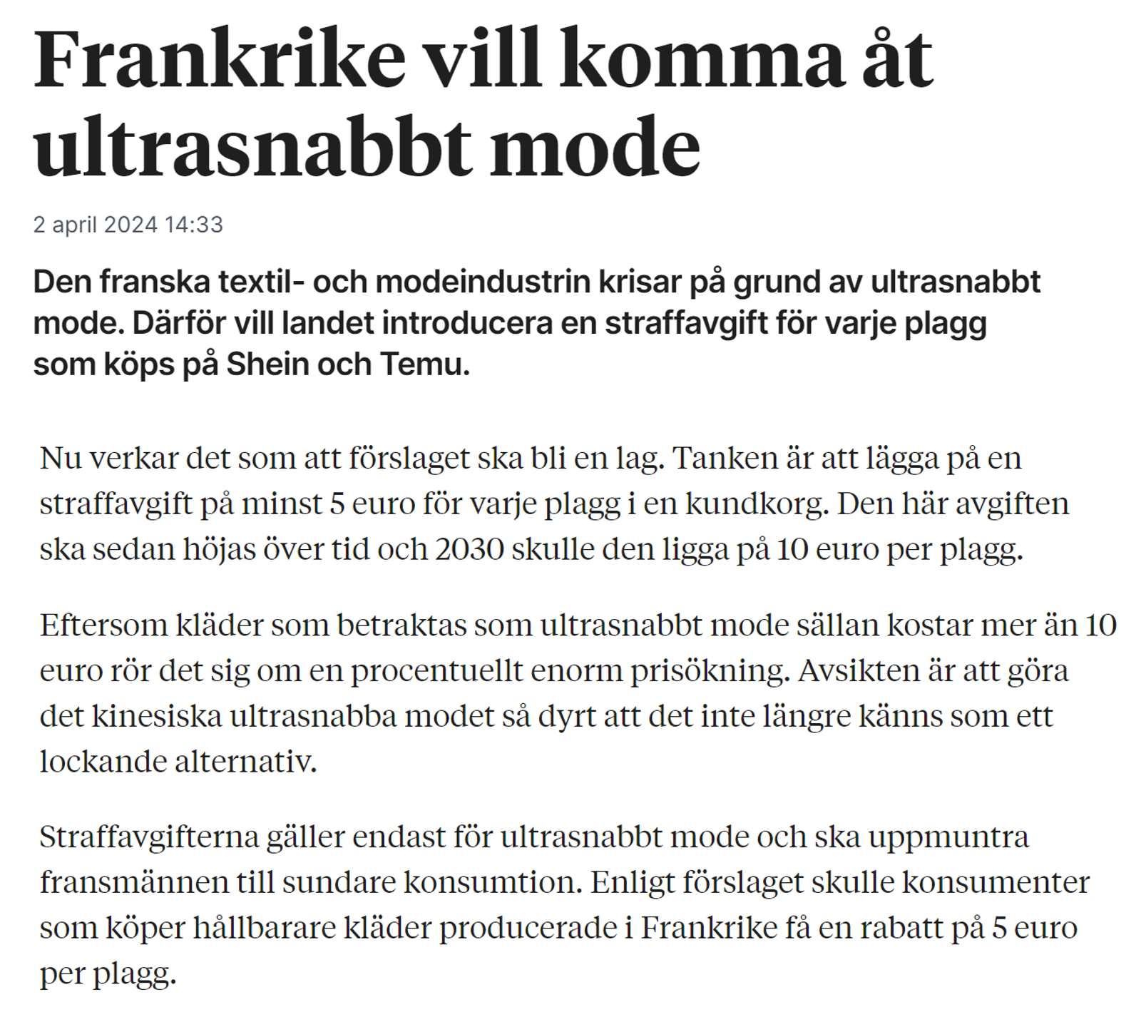
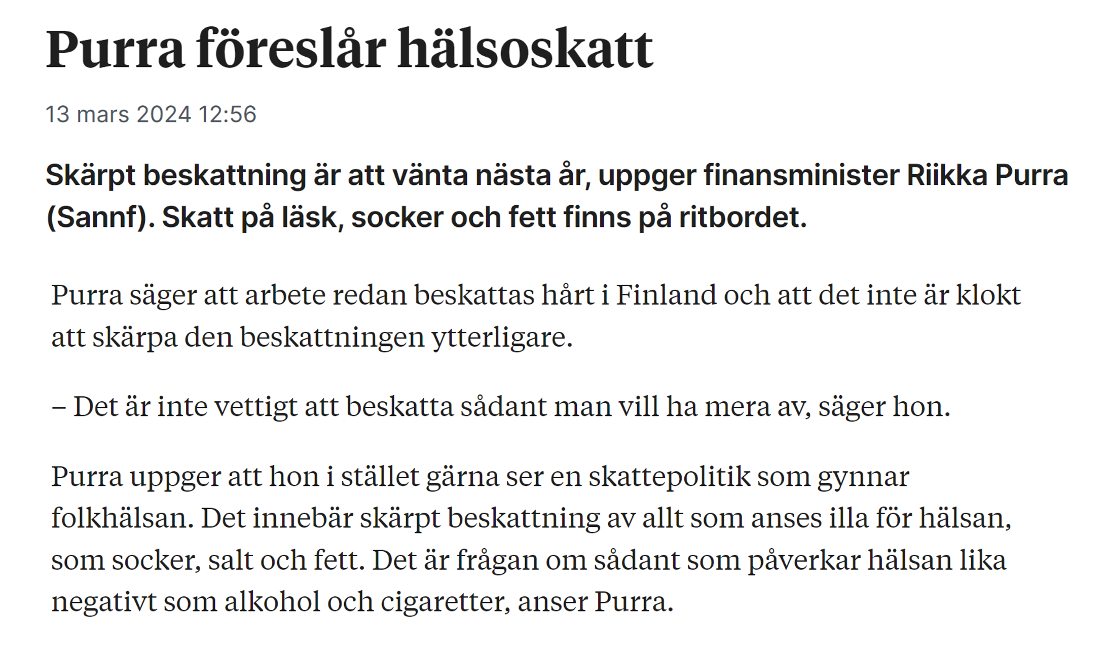
Here are some current examples of how economists and policymakers use taxes and subsidies to correct market failures:

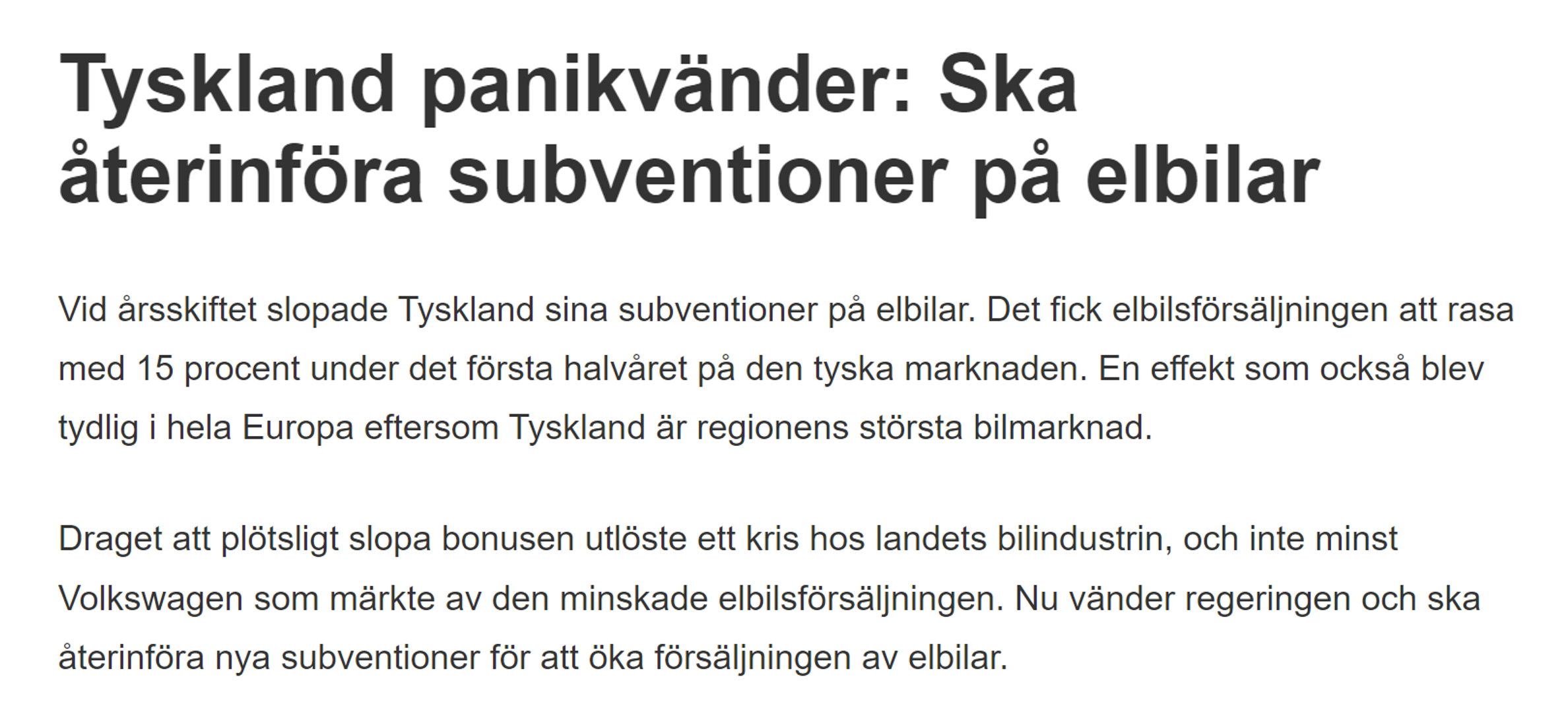
Remember that theory says taxes discourage and subsidies encourage. To see exactly how large the effects are you must look at the real world. What happened, for example, to EV sales in Germany when the subsidy was removed — and what happens now that it is reintroduced? Are differences in subsidies the reason 97% of new car sales in Norway are electric while the share is only 57% in Finland and 10% in the USA, or are there other explanations? What do you think?

Emissions trading

A third method to control pollution is emissions trading. The basic idea is:

Authorities decide how much may be emitted in total — for example 1,000 tonnes of CO₂.
They create emission permits — say 1,000 permits — where each permit allows one tonne of CO₂ emissions. The permits are then allocated to firms in any chosen way: everyone could receive the same number, or larger firms could be given more permits than small firms.
Suppose your firm, Åbo Paper, receives 100 permits. That means you may emit 100 tonnes of CO₂ at no cost.

At the same time authorities create a market where firms can buy and sell these permits, with prices determined by supply and demand. Environmentally friendly firms that do not need all their permits can sell their surplus to firms that find it costly to reduce emissions. This ensures emissions are reduced first where it is cheapest to do so, while green firms gain financially.

One advantage of tradable permits over taxes is political feasibility: environmental taxes hit all firms, while a cap‑and‑trade scheme can instead become a windfall for low‑emission firms. Cap‑and‑trade therefore appears likely to be the dominant global instrument for tackling climate change — perhaps the defining issue of our time. Below you first see a video explaining how the system works and its challenges, and then a chart of per‑capita emissions from 1750–2024. Where are emissions highest? Are emissions in Finland rising or falling? My tip, as always: play with the data and explore the world!

Solutions according to the Coase theorem

Besides using quotas, environmental taxes and emissions trading there is a fourth proposal for how authorities can deal with externalities. This solution is to do nothing. According to the so‑called Coase theorem, the market can in principle solve environmental problems by itself — but only under very specific conditions.

The following analogy may help you understand the Coase theorem: you farm wheat and rye on the fields outside Turku. The Helsinki train line also runs across the fields.

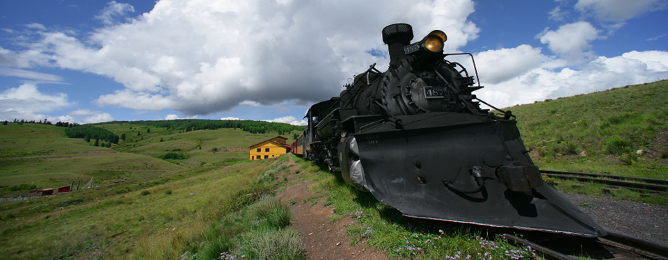
The problem is that when the train runs faster than 140 km/h sparks fly off the rails and sometimes these sparks set your crops on fire. Several times you have lost substantial sums, but the railway company doesn’t care a whit. For them the priority is getting passengers quickly to Helsinki and they have no incentive to slow down for your sake. What happens on the rail market therefore affects you, an outside party — a classic example of an externality. You beg the authorities to fix the problem, perhaps by imposing speed limits or a government fee equal to the damage caused by rail traffic.

Ronald Coase (1910–2013) argued, however, that the market can itself handle the problem without government intervention. Coase put it roughly like this:

“Bring together the party causing the externality and the affected third party and let them bargain to a mutually satisfactory solution. Given that property rights are clearly defined and transaction costs are zero, the market will reach an efficient outcome by itself despite the externality. This holds regardless of who is initially assigned the property right.”

Suppose, for example, it is clear that you own the land. In negotiations with VR you could probably find a compromise both sides can live with. If it is extremely important for VR to drive fast they might pay you a few thousand euros a year for the right to speed. If instead VR owned the land you could also reach an agreement: if it is crucial for you that no crop burns, you might pay VR compensation to drive slowly across the field. Who owns the meadow affects who receives the money, but in either case you should be able to bargain to an outcome that internalises the externality.

According to Coase, the authorities’ main task is therefore to secure and protect property rights. It must be crystal clear who owns the meadow. Transaction costs must also be low, meaning it must be easy for you and VR to meet, negotiate and sign a contract. Given well‑defined property rights and low transaction costs the parties themselves should be able to negotiate a solution that makes everyone better off.

But does the Coase theorem work in practice? In other words: can markets solve environmental problems without economists and policymakers intervening? Even Coase himself was highly sceptical. It may work for problems that are localized and clear — for example, when a factory dumps waste on your backyard. You plainly own the plot (property rights are clear) and you can easily meet the factory management (transaction costs are almost zero). But many environmental problems today are diffuse and global. In 2022 China emitted 11.2 billion tonnes of CO₂ into the atmosphere. Who owns the air, and how could all those affected possibly sit down at a negotiating table with every emitter and agree on a binding deal?

8.4 When price is missing

We will now go on a fishing trip with my father and attend a New Year’s party to discover two more cases where the market is not as good as we first thought.

Common resources. In the 1970s my father’s biggest hobby was fishing. Almost every evening he took the boat out to sea to catch pike. According to him, he emptied large parts of the Stockholm archipelago of fish. No one could stop him from fishing. When I went pike fishing in the Baltic Sea last summer I hardly ever got a bite. The few fish I hauled up were unimpressive. My fishing trips were often failures. Everybody was disappointed and the kids cried.

Example of common resources: My father empties the Baltic Sea in the summer of 1977

Public goods. On New Year’s Eve I attended a big party. I didn’t bother to bring fireworks, even though I love them. Coldly rational, I assumed at least some other guests would bring rockets so I could enjoy their display. Nobody can stop me from watching the sky. At midnight everyone gathered outside in the dark. The children were excited. But it was a fiasco: almost no one had bought fireworks. The few rockets that were launched were unimpressive. It was a very sad start to the new year. Everyone was disappointed and the kids cried.

Why did the pike disappear from the Baltic Sea and why were there no fireworks? We will examine this more closely now. Let’s start with some definitions that help us think about the issue. In the table below I have classified goods according to two questions: Is the good excludable? Is the good rivalrous in consumption?

	RIVAL IN CONSUMPTION	NONRIVAL IN CONSUMPTION
EXCLUDABLE	Private goods Ex: Coffee, strawberries Can charge a price, markets work	Artificially scarce goods Ex: Music, film (paywalled) Can charge but MC≈0 can lead to under‑provision if priced poorly
NON‑EXCLUDABLE	Common resources Ex: Pike, clean air Cannot easily exclude users + rivalrous consumption leads to overuse	Public goods Ex: Fireworks display, lighthouses, public e‑book access Non‑excludable and non‑rivalrous → markets may not provide them

Table 8.2: Four types of goods

In the upper‑left quadrant we find private goods, which are both excludable and rivalrous. A cup of coffee is a typical example. That the coffee is excludable means the Astra café can stop you from drinking it unless you pay. Excludability makes it possible for the café to charge a price, so markets often work well for these goods.

But what about goods that are non‑excludable? When no one can be prevented from using them it becomes virtually impossible to charge a price. Why would anyone pay €10 for something they can use for free? Let’s explore these non‑excludable goods a bit further.

Common resources: The pike that disappeared

Why did the pike disappear from the Baltic Sea, and how can we fix it? Common resources are non‑excludable and rivalrous. Think of fishing in the Stockholm archipelago in the 1970s. In practice anyone could go fishing. My father could freely take his boat out every evening and fill it with pike. Fishing is also rivalrous: when my father eats one pike there is one fewer fish left for the rest of us to catch. A good being rivalrous means one person’s consumption reduces others’ opportunities to consume the same resource. But my father had no economic incentive to limit his fishing to preserve the stock. This fundamental problem means that other common‑pool resources — clean water, fresh air, public beaches, publicly owned forests and mountains — also tend to be overused.

So how do we prevent overuse of common resources? There are strong arguments for government intervention — limits on fishing, fishing licences or car tolls to protect the environment. Some economists, however, argue that commons can sometimes be protected without state intervention. To see why, let’s visit a meadow outside Turku.

The tragedy of the commons. You live in a small village where many people own sheep that graze on the village common, “the commons.” You are thinking of getting one more sheep. The benefit — more milk and wool — accrues to you alone, while the cost — pasture degradation — is shared by all villagers. From a selfish point of view it may therefore pay you to expand your flock. “If I don’t add sheep, the neighbours will anyway,” you might reason. Because everyone thinks the same way, the commons ends up with so many sheep that the pasture is trampled and the animals starve. That is indeed a tragedy.

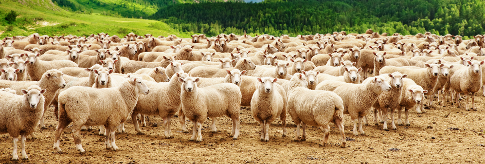
The problem here is the lack of incentives to care for a jointly owned resource. One solution is therefore to privatise the resource, which forces each owner to internalise all the costs of their actions. Over‑exploiting the pasture would then hurt your wallet. Previously it was mostly the other villagers who paid the price for your unsustainable behaviour. Non‑excludability — and thus free access — often stems from the absence of clear property rights. If the lake were owned by someone, that owner would have an incentive to protect the resource and explore alternative uses, such as tourism. That way you might have been able to stop my father’s pillaging of the Baltic Sea in the 1970s.

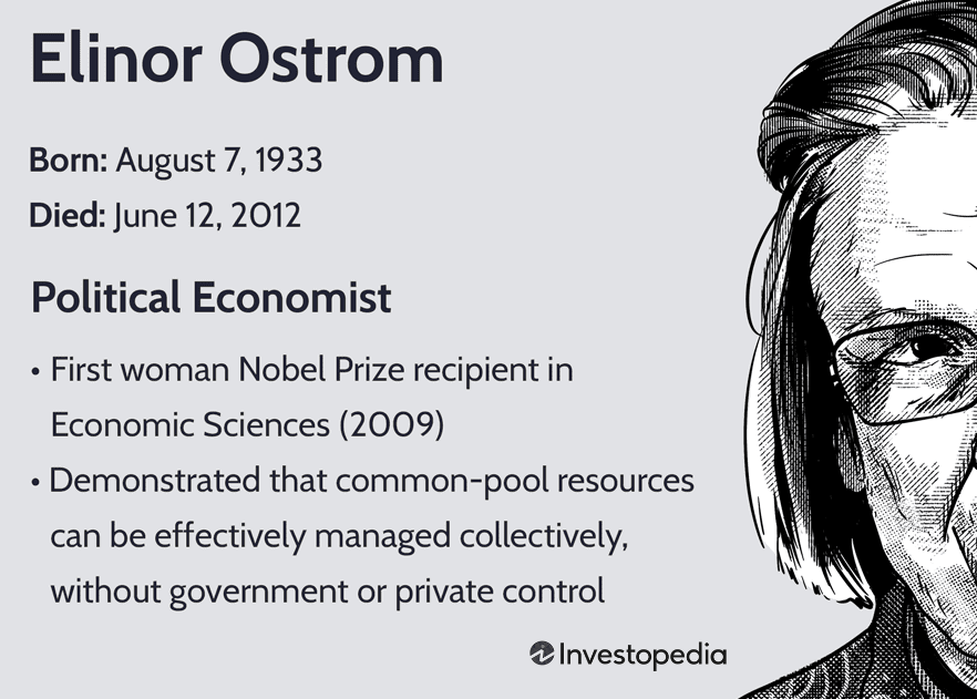
Other economists, such as Nobel laureate Elinor Ostrom, argue that commons are not destined to be over‑exploited. She maintains that social norms can protect resources. Peer pressure and solidarity with your neighbours can, Ostrom argued, allow the meadow and the sea to thrive. The question is whether these social norms are strong enough when the resource is owned not just by your neighbours but by everyone on the planet — such as the air and the oceans. That challenge makes climate change even harder to handle than many other, more local environmental problems.

Economists know what can be done, in principle, to tackle global warming and marine eutrophication. In practice, however, political reluctance to implement the necessary measures has been strong. It is a political failure that leads governments to shift the problem onto other countries and onto future generations.

Public goods: Fireworks and lighthouses

Finally, let’s examine the lower‑right quadrant in Table 8.2. What happens when a good is both non‑excludable and non‑rivalrous?

Fireworks are an example of a public good. Think back to my New Year’s party. Why were the fireworks so poor? Because nobody can be prevented from watching the sky. This non‑excludability means no one will pay for something they can enjoy for free. The fact that it’s free to watch fireworks means few people are willing to buy them — so the market provides only a small display. The same problem arises for other public goods such as lighthouses, national defence or this e‑book. Imagine you are sailing in the archipelago on the night of a nuclear accident. You can listen to the emergency broadcast that goes out across Finland without paying. You can also navigate home by the light from the lighthouses without paying. Your listening to the broadcast and using the lighthouse does not reduce other Finns’ ability to do the same at the same time. This e‑book is also an example of a public good: no one can be prevented from consuming it, and your reading it does not reduce others’ ability to read it.

Markets typically fail to provide the right quantity of public goods. Who would produce something if they cannot charge for it? That is why government intervention is often well justified. In practice it is usually the state or municipalities that pay for public goods such as our defence, basic research, roads, public art and the New Year’s fireworks displays. In an exercise at the end of the chapter you will consider how politicians can decide how much of a public good to produce.

public goods are goods that everyone can use and that are not consumed by a single person at a time but benefit many users simultaneously, for example a fireworks display or this e‑book

Exercises

In this chapter you learned why markets fail when market activities also affect people outside the market. If you understand these externalities, you will also understand why many environmental problems arise — and how to tackle them with smart economic policies. Below are some cases where you can apply your knowledge in practice. Press Show Answers when you want the computer to grade your responses. Good luck!

The airline industry and global warming

Every month many Finns fly the Helsinki–London route. Several airlines operate the route, so you can assume the market is characterised by perfect competition. The inverse demand is given by $\small P_D=800-0.05Q$ while the inverse supply is $\small P_S=20+0.025Q$, where Q is the number of passengers and P is the ticket price.

The price of a plane ticket to London will be and the number of tickets purchased will be .
Each person flying to London causes a negative externality equivalent to €60. What would be the socially optimal number of Helsinki–London trips? Answer: .
As environment minister you introduce an air travel tax of €30 per trip. What becomes the new consumer price to fly to London? Answer: .
The Coase theorem says the market can be efficient even with externalities, but only if two conditions hold. What are these two conditions and do you think they hold in the Helsinki–London air travel case?

Hints here.

Review Chapter 3 if you are at all unsure how to solve this problem or how to draw supply and demand in a diagram.
Think of the current supply curve as reflecting only firms’ private costs. The “optimal” supply curve should reflect all costs — both firms’ costs and third‑party costs. So raise the original supply curve by the size of the externality. Then solve $\small 800-0.05Q = 80+0.025Q$ to find the socially optimal quantity.
Set $\small P_S+30 = P_D$ and solve for how many tickets are sold (you should get 10,000). Use the demand curve to read off what consumers are willing to pay.
Read.

Plastic pollution

A major environmental problem in the world is plastic pollution.

Using the world map above (click Table and sort with the arrows) I see that the country that dumped the most plastic into the oceans per person in 2019 was .
The country that was the correct answer above emitted a total of 356,371 tonnes of plastic into the oceans in 2019. A large share consisted of single‑use plastic, for example bags and plastic packaging that come with other purchases. Imagine the market for soft drinks in a small coastal town. Daily demand for 1‑litre PET bottles of soda is $\small Q_D=40{,}000-200P$, where Q is the number of bottles and P is the price per bottle in Philippine pesos. Supply is $\small Q_S=200P -4{,}000$. The number of bottles sold each day is therefore .
Each PET bottle imposes a negative externality of 40 pesos. What would be the socially optimal number of bottles sold? Answer: .
The market price of the soda — 110 pesos — is too low because it reflects only the firms’ private costs and not the environmental damage caused by the plastic bottles. The price per bottle that would lead to the socially optimal quantity of soda would be .

Hints here.

Click Table to see the data more clearly. Sort by clicking the arrows.
Practice drawing the exact curves in a diagram.
It’s easiest to work with the inverse functions here. $\small Q_D=40{,}000-200P$ can be rewritten as $\small P_D=200-0.005Q$ and $\small Q_S=200P -4{,}000$ can be inverted to $\small P_S=20+0.005Q$. Now shift the supply curve up by the size of the externality so that the new supply curve reflects both the firms’ costs and the third‑party cost. How much would be produced if firms were required to take the negative side effect into account?
What would consumers be willing to pay for the socially optimal quantity of soda? That is the price policy should aim for (for example via a tax).

Yes or no to a plastic bag tax

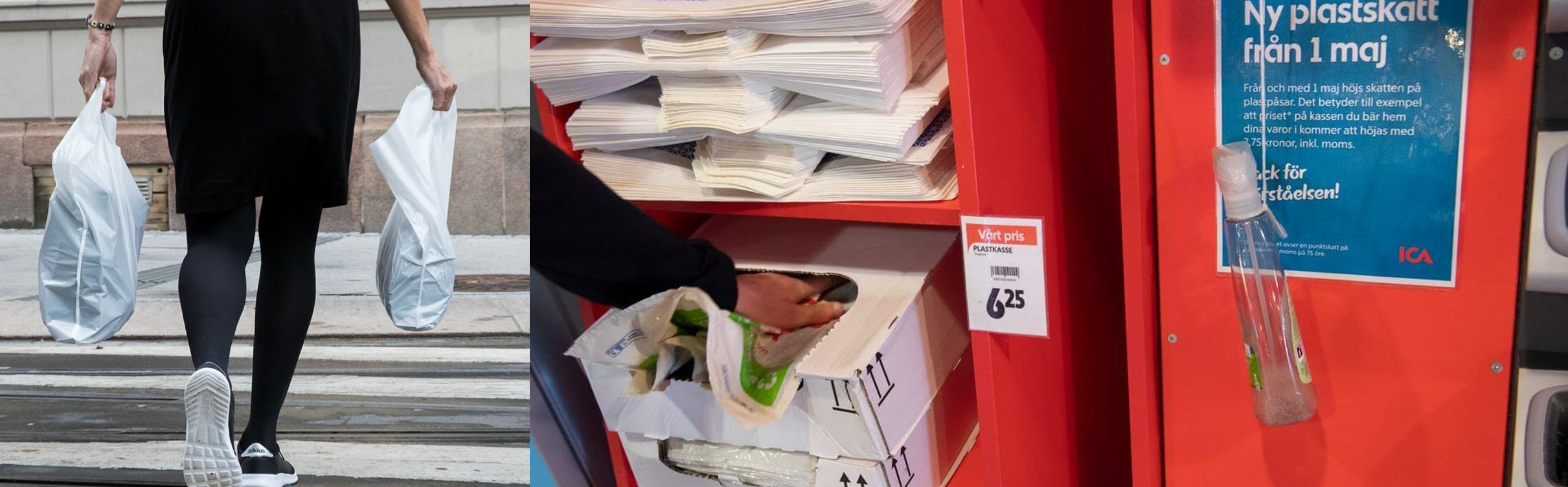
Swedes use far fewer plastic bags today. In 2017 Swedes used 83 plastic carrier bags per person; by 2023 that number had fallen to 15. A likely contributing explanation was the plastic‑bag tax introduced on 1 May 2020. Each bag was then taxed by about three kronor.

Draw a diagram of the market for plastic bags and explain why the market outcome leads us to consume more bags than is socially optimal.
Show in the diagram how a plastic‑bag tax brings consumption down to the socially optimal level.
Would it be better to ban plastic bags altogether (i.e. reduce consumption to zero)? Argue from economic theory.
The tax is repealed on 1 November 2024. What will happen to the price and the quantity of bags?

Hints here.

Think about what the supply curve actually reflects. Does it include the third‑party cost?
Think about how a tax affects the analysis. Remember that taxes reduce quantity, so check that quantity falls once you include the tax. The consumer price should also rise, so verify your diagram agrees with common sense.
Practice writing your answer on paper so you won’t be doing this for the first time under exam pressure.
What happened when the tax was introduced? When it is repealed the opposite will, of course, occur.

Emissions trading

Suppose two firms in a town together emit 80 tonnes of CO₂. The city now decides that annual emissions must be halved to 40 tonnes. The question is how to achieve this. For one firm, UPM‑Kymmene, it always costs only €10 to reduce emissions by an extra tonne. For the other firm, Stora Enso, it is considerably more costly to cut emissions.

Firm	(1) Do nothing!	(2) Halve emissions
UPM‑Kymmene	Emits: 40 tons
Cost to reduce: €10/ton	Emits: 20 tons	Receives 20 emission permits
Stora Enso	Emits: 40 tons
Cost to reduce: €40/ton	Emits: 20 tons	Receives 20 emission permits

Right now (1) the firms emit a total of .
Politicians now propose strategy (2), where each firm must halve its emissions. UPM‑Kymmene therefore needs to reduce emissions from 40 to 20 tons. According to the table, what does it cost UPM‑Kymmene to halve its emissions? Answer: .
According to the table, what does it cost Stora Enso to halve its emissions? Answer: .
What is the total cost of halving emissions this way? .
As an economist you instead propose strategy (3), a system of tradable emission permits. Each firm receives 20 permits, where each permit allows 1 ton of emissions. Firms can trade permits among themselves. Suppose the price per permit is €30. UPM‑Kymmene reduces emissions to , which costs them , and instead sells its 20 permits at €30 each, generating revenues of . Stora Enso, however, does not reduce emissions at all but buys 20 permits from UPM‑Kymmene for €600.
Halving emissions via direct regulation (2) cost €1,000. What is the cost of halving emissions instead via tradable permits (3)? .
Reducing emissions more cheaply is clever and also benefits firms that are good at cutting emissions. How is UPM‑Kymmene affected economically by switching from (1) to (3)? Answer: .
How is Stora Enso’s economy affected by switching from (1) to (3)? Answer: .

Hints here.

Play until you understand how the system works. The central lesson is that the “rigid, bureaucratic” way of reducing emissions is far more expensive than a market‑based solution.

Positive externalities and the cholera vaccine

So far we have mainly studied how society is affected by negative externalities. But what happens with positive externalities? Play with the app earlier in the chapter. Think like this: a positive externality means that not only the consumer benefits from the good or service but also a third party outside the transaction. In the app I have therefore included an “Optimal demand” curve that captures not only the consumer’s benefit but also the benefit to the third party. You can think of a positive externality as shifting the demand curve up by the size of the externality. With positive externalities market production is therefore too small from a social perspective. If taxes were a way to curb excessive production in the case of negative externalities, then subsidies to firms are a natural way to increase production of goods and services that generate positive externalities.

Cholera is a very serious gastrointestinal disease spread through contaminated drinking water. Each year nearly 3 million people are affected by cholera and almost 100,000 die. The map below shows the share of newborns who die before age five.

Using the world map above (click Table and sort with the arrows) I see the country with the highest under‑five mortality in 2024 was .
Of 100 children born in Sweden in 1751, on average died before age five.
Has child mortality increased in any country since 1960? .
Will the market (without government intervention) produce the socially optimal quantities of alcohol and flu vaccines? Argue clearly.
Patents make cholera vaccines expensive. Do you think patents for cholera vaccines are wrong?
Linda works on saving children in Botswana. Suppose demand and supply for cholera vaccine per year are $\small Q_D=800{,}000 - 2{,}000P$ and $\small Q_S=-400{,}000+2{,}000P$, respectively, with P in dollars and Q the number of doses. Under competition, how many doses will be traded? .
Each vaccine dose generates a positive externality of $140. The socially optimal number of doses would therefore be .
Linda persuades Botswana’s politicians to subsidise the vaccine so the socially optimal quantity is reached. The total cost of the subsidy is and the consumer price at the clinic becomes .

Hints here.

Play and explore.
Another tip: check child mortality in Finland in 1868. Is this a data error or did something special happen in Finland that year? See the YLE article here.
No — child mortality has fallen in every country worldwide since 1960.
The easiest way to answer these questions is probably to draw a supply‑and‑demand diagram and mark how much the market supplies. Then show the socially optimal output when there are negative or positive externalities. Explain in one or two sentences why the market fails.
Show that the vaccine quantity on an unregulated market is inefficiently low (because of positive externalities). A subsidy can increase production. Remember, however, that huge R&D investments are often needed to develop a vaccine. The market price may be so low that no firm dares to try. A patent grants monopoly profits for 20 years, which can encourage firms to attempt vaccine development.
Set supply equal to demand.
It is easiest to work with the inverse functions here: $\small P_D=400 - 0.0005Q$ and $\small P_S=200 + 0.0005Q$. Each dose yields an additional positive externality of $140$. Think of the demand curve as showing the private benefit to the consumer, but now add the extra $140$ of third‑party benefit. Shift the original demand curve up by 140 and find the new equilibrium: $\small P_D+140=P_S$ gives $\small 540-0.0005Q=200+0.0005Q$. Solve for Q to find the socially optimal quantity.
Now take that socially optimal quantity and multiply it by 140 to find the total value of the external benefit.

How to save our common resources

Much of nature can be described as common‑pool resources. Because they are non‑excludable no one can be prevented from using them. They are also rivalrous: when you pull a pike from the lake or cut down a tree in the forest you reduce other people’s opportunities to fish or use the woodland. Because you do not have to take into account the harm your behaviour imposes on others, there is a strong risk that common‑pool resources will be over‑exploited. The map below shows the annual change in forest area over the period 1991–2025:

In which country did the most forest disappear in 2025 (measured in hectares)?
In Brazil, Indonesia and Tanzania the rainforest is being cleared. There are many explanations for this deforestation. Research has shown that important drivers include expanded industrial agriculture, overexploitation of timber, increased urbanisation and climate change. There is also a clear link between strong property rights and reduced deforestation. Explain, using economic theory, why deforestation is likely to decline when it is clear that someone owns the rainforest (whether the state or private actors).

Hints here.

Note how much forest is lost in the tropical regions.
If someone clearly owns a resource it becomes harder to over‑exploit it. If ownership of a rainforest is unclear you can cut it down to build on it; if the state (or a private owner) clearly owns it, this becomes much harder. Many environmental problems stem from the absence of rules, institutions and property rights. You will learn much more about these issues in the Environmental Economics course.

How many lamp posts should there be in the park?

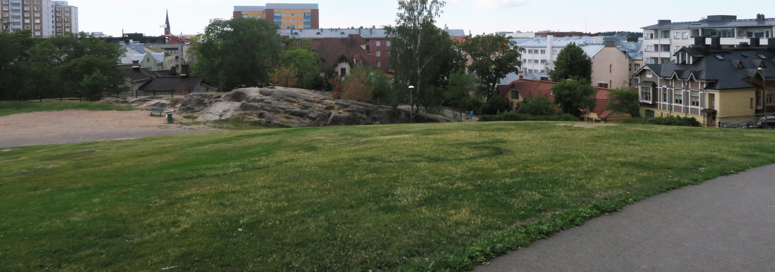
Puolala Park, a stone’s throw from the Market Square, is perhaps Turku’s most beautiful park. At night, however, it can feel a little spooky. Many people therefore demand more street lighting in the park. Street lighting is an example of a public good, because lighting is both non‑excludable (everyone can benefit from it) and non‑rivalrous (your use does not reduce mine). The question is only how many lamp posts should be installed in the park. Since you have studied economics at university level, you are the one who has been asked to investigate the issue.

Why does the market (without government intervention) fail to produce the correct quantity of public goods?
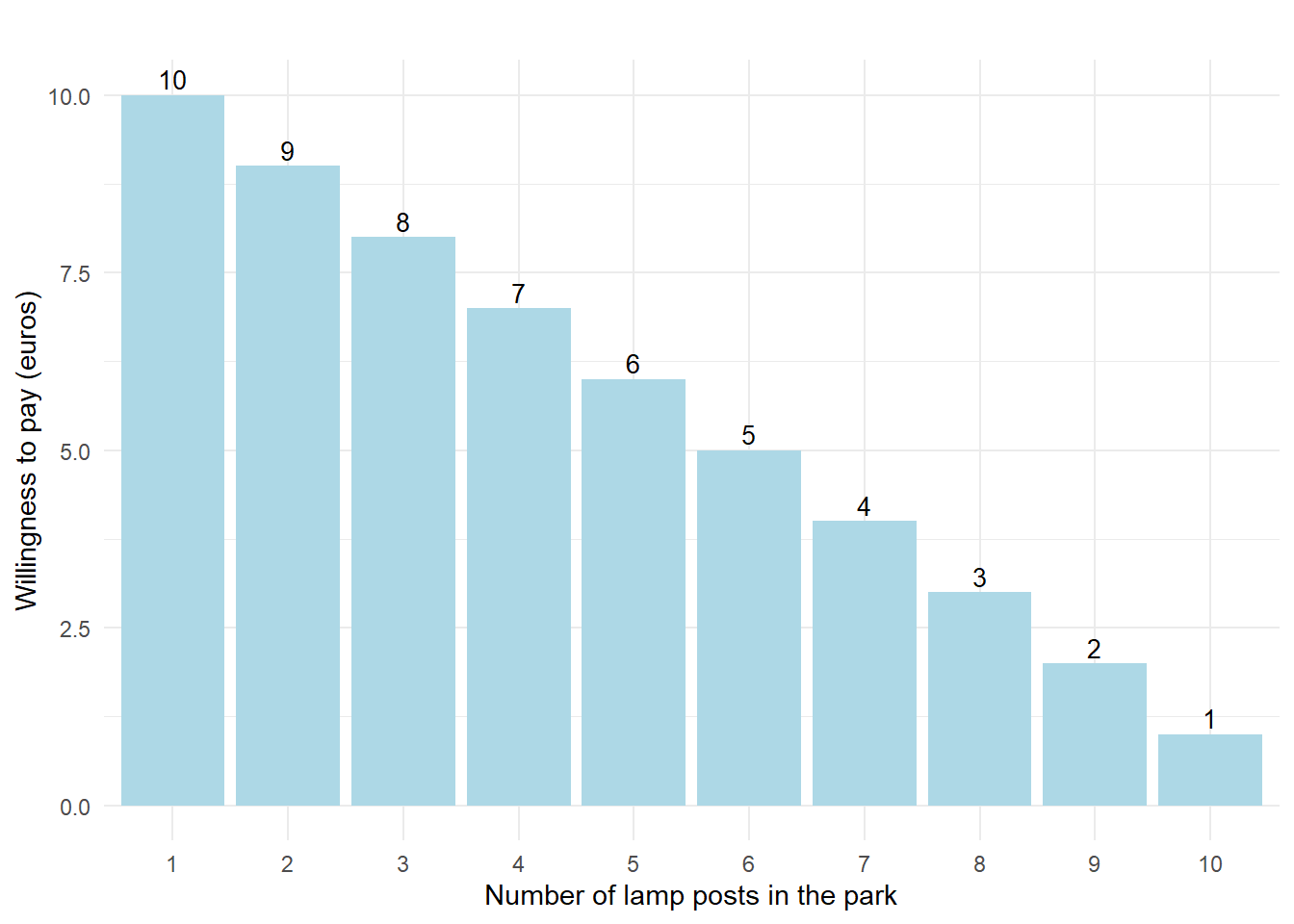
Your first step is to interview some Turku residents who use the park to ask how much they value lighting. You quickly find that the figure below seems typical for how an individual values lighting. How do you interpret the figure?

Assume there are in total 1,000 Turku residents who use the park annually. The cost to install and maintain one lamp post for a year is €3,000. How many lamp posts should the municipality install in the park?
Is there a risk that your interviewees overstate their willingness to pay? Explain!

Hints here.

Public goods are non‑excludable — no one can be prevented from using them without paying. That makes it impossible to sell these goods. Which firm wants to produce something it cannot charge for? A pure market therefore will not provide public goods. Instead it falls to the state and municipalities to fund our public goods.
Imagine you were the interviewee. The figure shows how much you value each lamp post. The bars indicate that you value every extra lamp, but the first lamp is by far the most valuable: you assign it €10. Picture the park in total darkness — the first lamp lights the path and makes it possible to walk through the park at all. A second lamp is also very useful, but not as crucial as the first. The tenth lamp you value at only €1 — once nine lamps are installed the whole park is lit, so lamp ten is hardly essential.
Light from the lamps is non‑rivalrous. Your consumption of the light does not reduce my ability to enjoy the same light. This means we can multiply the per‑person values in the chart by 1,000 users. The residents collectively value lamp 1 at €10,000, lamp 2 at €9,000, and so on. As a municipal official you should install lamps until the last lamp’s social benefit equals its cost. The optimal number of lamps in the park is therefore eight.
Imagine the interview situation in the park. If you claim a very high willingness to pay, that will likely lead to more lamps being installed — but the bill is passed on to taxpayers.

For those who want to know more:

Ekonomistas is a good Swedish‑language blog where economists discuss society, politics and scholarship.