4 Why income inequality?
(where you learn methods to figure out why some people earn more than others)
So far you have learned how a market works. You can use the principle of supply and demand to understand all kinds of trading, whether it’s strawberries, stocks — or people. The same rule applies in the labour market: “things that many want and that are hard to produce tend to be expensive.”
If you possess unique skills that many employers demand you can expect a high wage. Yet it is sometimes hard to understand why some people earn more than others. Is it about education? Or where they live? Maybe they sacrificed their private life? Or is the explanation something entirely different?
In this chapter you will see how some of the recent Nobel laureates in economics have approached solving this puzzle.

4.1 The research challenge
Imagine the student associations MK and SF launch a project called Evening Study. Every Wednesday evening anyone can come to a classroom to study in a calm, quiet environment. The associations provide coffee and fresh buns, and experienced tutors are on hand to help you.
The rector quickly becomes interested in the project. Students doing well is of course great for them, but as we saw in Chapter 1 successful students are also a goldmine for the university. But has the project actually improved students’ study results? And if so, by how much have the results improved?
You will encounter this type of challenge often, both during your studies and in working life. So how do you solve it? My advice is to think back to Figure 1.1, where we saw that there are several possible paths through life. In this situation you can think of the left path as participating in Evening Study, while the right path shows what happens to your study results if you do not participate in Evening Study.
To evaluate the project the rector turns to Bill Murray. Bill is particularly well suited for the task because he has a unique ability to see how different choices affect people’s lives:
Bill Murray in “Groundhog Day” can go back in time and see the outcome along The Road Not Taken.
The ability to travel in time would allow Bill to collect the following data:
| Student | Score if attending Evening Study | Score if not attending Evening Study | Effect of attending Evening Study |
|---|---|---|---|
| Anton | 27 | 24 | +3 |
| Benjamin | 6 | 5 | +1 |
| Clara | 21 | 19 | +2 |
| Daniela | 27 | 26 | +1 |
| Edvin | 21 | 19 | +2 |
| Frida | 18 | 15 | +3 |
| Average: | 20 | 18 | +2 |
At the top of the table is the student Anton. Thanks to his time trips Bill can see that Anton scores 27 points on the exam when he attends Evening Study but only 24 points when he does not. Hence Bill can conclude that Evening Study gives Anton 3 extra points on the exam. The table similarly shows the effect for other students. For example, Evening Study raises Benjamin’s result from 5 points to 6 points. On average these voluntary evening study sessions increase scores by 2 points per student, which corresponds to almost half a grade. Not bad!
Unfortunately Bill Murray declines the rector’s offer. Instead you are given the task of evaluating the project. Since you cannot travel in time, however, you can only collect the following data:
| Student | Score if attending Evening Study | Score if not attending Evening Study | Effect of attending Evening Study |
|---|---|---|---|
| Anton | 27 | - | - |
| Benjamin | - | 5 | - |
| Clara | - | 19 | - |
| Daniela | 27 | - | - |
| Edvin | 21 | - | - |
| Frida | - | 15 | - |
| Average: | 25 | 13 | - |
Anton, Daniela and Edvin attended Evening Study, so you only see how they performed when they attended, not how they would have done had they stayed away. Benjamin, Clara and Frida did not attend, so we can never know how they would have fared on the exam if they had participated. All we observe is that attendees Anton, Daniela and Edvin averaged 25 points on the exam, while non‑attendees Benjamin, Clara and Frida averaged only 13 points.
Many would probably interpret these results like this:
Huge success when the student associations organised evening study! Exam scores almost doubled — from 13 to 25 points. Tutor‑led evening sessions seem to help students more than anything else. Expanding the programme massively and making evening study compulsory would be a brilliant initiative that would benefit students, the university and society at large.
But as you know, this conclusion is wrong. The true effect of Evening Study was an increase of 2 points, not 13. Making the programme compulsory would therefore hardly cause exam scores to soar. So why did this misperception arise?
The problem is that students were allowed to choose whether to participate. That means there may be other differences between participants and non‑participants that affect outcomes. Perhaps Anton, Daniela and Edvin are highly ambitious students, while Benjamin, Clara and Frida take their studies more lightly. The fact that attendees did well on the exam thus reflected the type of students who showed up, not primarily the effect of the programme itself.
How can we avoid this problem? Because the difficulty arises when students choose, one solution is to ensure they cannot choose. Instead, participants could be selected by lottery. The lucky ones receive extra study support, while the unlucky miss out. If participants still perform better than non‑participants under random assignment, this would be credible evidence that Evening Study truly improves outcomes. You could no longer attribute the difference to attendees being more ambitious to begin with.
Random assignment can, however, be problematic and may feel unfair or unethical. Sometimes — entirely naturally — situations arise where your path through life is determined by chance. In the rest of this chapter we will study some such interesting cases to better understand the labour market. Imagine yourself sitting at the Market Square in Turku watching people pass by — and trying to understand why some earn more than others. Let your imagination run wild!
4.2 War experience and income
War can leave deep scars on those forced to endure it. For example, over half a million Finns fought in World War II and three million Americans served in Vietnam, and the question is whether such wartime experiences leave lasting trauma that affects how you fare on the labour market later in life. We will therefore examine how war affects future income, with a special focus on Americans who fought in the Vietnam War. How did they actually fare after returning home?
To understand the challenge I have the following somewhat provocative tip: For once, let your dusty stereotypes run wild! Close your eyes and imagine an American who voluntarily enlisted to fight in Vietnam in the 1960s. What do you see?
Perhaps you picture “a jobless, low‑IQ troublemaker who dropped out of school at 13”? If veterans like these turned out to have low incomes in the 1980s that would not be surprising — such individuals often struggle in the labour market regardless of whether they fought in Vietnam. Or maybe you imagine “a charismatic, stress‑resistant leader who answered the call of duty and never backs down”? If these people later earned higher incomes that would also not be strange — they might have succeeded in their careers even without combat experience.
This thought experiment illustrates the difficulty of deciding how the Vietnam War affected later incomes. It is possible, even likely, that those who chose to fight were different from those who did not — and those preexisting differences could themselves explain later income gaps.
But Joshua Angrist Angrist (1990), who won the Nobel Prize in Economics in 2021, found a clever way to get around this problem. Watch the short video clip below and you’ll understand:
The effect of Vietnam on future income. Lottery draw broadcast live on American TV in 1969 determining who was compelled to register for service in Vietnam — and how life later turned out for the veterans.

In December 1969 the U.S. authorities held a lottery to decide who would be called up for the war. Millions of young men watched anxiously as their fate was determined on live TV. The first date drawn was “14 September.” Anyone born on 14 September was therefore extremely unlucky — they were among the first to be called up. The last date drawn, slip 366, was “8 June.” Those born on 8 June were extraordinarily lucky and escaped Vietnam.
Angrist exploited this lottery in his study. His results looked like this:
| Drafted to conscription | Not drafted to conscription | Differences | Effect on 1981 earnings of having served in Vietnam | |
|---|---|---|---|---|
| Income 1981 (dollars) | 16,025 | 16,461 | -436 | -2,741 dollars |
| Share who actually served in Vietnam | 42.6 % | 26.7 % | +15.9 |
The table shows that those unlucky enough to be drafted had annual earnings about 10 years later that were $436 lower than those lucky enough not to be drafted. In other words, serving in the Vietnam War led to lower future earnings. Because draft lottery assignment was random, these results are hard to explain away by preexisting differences between the groups.
Being called to the draft did not automatically mean you served in Vietnam; the medically unfit were screened out at draft boards, and people with powerful parents sometimes found ways to avoid service. Also, those not drafted could still volunteer. But the lottery did affect the probability of serving in Vietnam. Since a 15.9 percentage‑point increase in that probability reduced annual earnings by $436, Angrist concluded that a 100 percentage‑point increase would reduce earnings by $2,741 (computed as 436 / 0.159).
4.3 Do studies pay off?
That some people earn more than others may also be because they have invested in more education. A good education makes you more productive — and employers tend to reward skilled people. But do you really earn more by studying? The figure below shows what Finns actually earn per month:
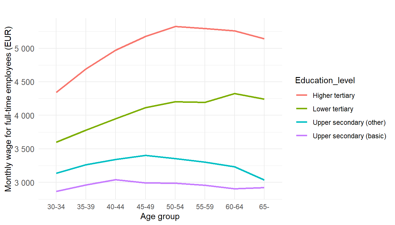
Finns aged 30–34 with a higher tertiary degree therefore earn about €4,350 per month, while people of the same age with only upper‑secondary education earn €3,100. A naive observer would likely conclude that a university degree raises your monthly wage from €3,100 to €4,350 — about a 40% increase.
mean wage is the average of everyone’s wages
median wage is found by lining up all Finns by wage (highest first, lowest last) and picking the person in the middle; that person’s wage is the median
human capital is the knowledge, skills and experience that make you productive
But what if those who chose to study were different from those who chose not to study? Again: let your stereotypes blossom! Maybe university students were already smarter and more ambitious at 17 — and perhaps it’s their high IQ and drive that explain the higher wages, not the studies themselves? Or maybe the opposite is true: those who didn’t continue studying were so talented that they did fine without Åbo Akademi (after all, neither Leo Messi, Bill Gates nor Taylor Swift hold master’s degrees), while university is mostly a place for lost souls who wouldn’t survive a single day in the real world?
To get around this problem we could, in principle, randomise who is allowed to study and who is not. David Card Card (1995), also a Nobel laureate in economics, found however a quicker and less ethically fraught way to measure the causal effect of education on wages. The figure below illustrates how Card cracked the puzzle:

There are thousands of schools in Finland. If you’re lucky, the nearest school is very close; if you’re unlucky, the commute is long. It’s almost as if you wake up one morning and — as in a lottery — find that a school has been built across the street, while your friend wakes up to discover she has an awful long way to the nearest school. Maybe that makes you study while your friend doesn’t. This is what the results looked like in the American study:
| Grew up near a school | Grew up far from a school | Differences | Effect on wages of one school year | |
|---|---|---|---|---|
| Hourly wage (log) | 6.31 | 6.26 | +0.05 | +15.6% |
| Years of schooling | 13.58 | 13.26 | +0.32 |
Note that those lucky enough to grow up near a school earned 5% more as adults than those who lived far away (a change in a logged variable can be interpreted as a percentage). Those who lived near a school also completed 0.32 more years of schooling. If 0.32 extra years raises wages by 5%, then one whole extra year of schooling would logically raise wages by about 15.6% (5 / 0.32).
But as a university student you may be most interested in how higher‑level studies affect your wallet. What would happen to your wage if we suddenly cut 20% of an education programme — roughly 12 courses of 5 credits each? We can explore this in the data. Exactly such a radical change took place in 2006 at Colombia’s top university — and Arteaga et al. (2018) show that the reform reduced the wages of graduating economists by 16%. The reason, the researchers argue, was that students who completed the reduced curriculum found it much harder to access high‑paying sectors and employers. Maybe keep this in mind next time your motivation falters: if cutting 12 courses reduces wages by 16%, then one course is associated with roughly a 1.33% wage increase. So by taking one extra course a monthly salary of €4,000 could rise to about €4,053 — about €636 a year. Accumulated over a long career, that adds up to a lot of money (at least it did for economists at a leading Colombian university in 2006).
4.4 Born a leader?
Education seems to raise incomes, and one possible reason is that it increases the chance of becoming a manager. The School of Economics at Åbo Akademi aims to “educate creative, critical‑thinking, responsible leaders”. But can leadership really be taught, or are leaders born?
Grönqvist et al. (2015) studied a situation where chance determines who receives leadership training, and they use this to investigate whether leadership can be learned. The trick was to dig deep into data from Swedish draft boards. In the figures below the horizontal axis shows how the young men performed on various tests at military conscription, while the vertical axis shows the probability of holding a managerial position at ages 30–40.
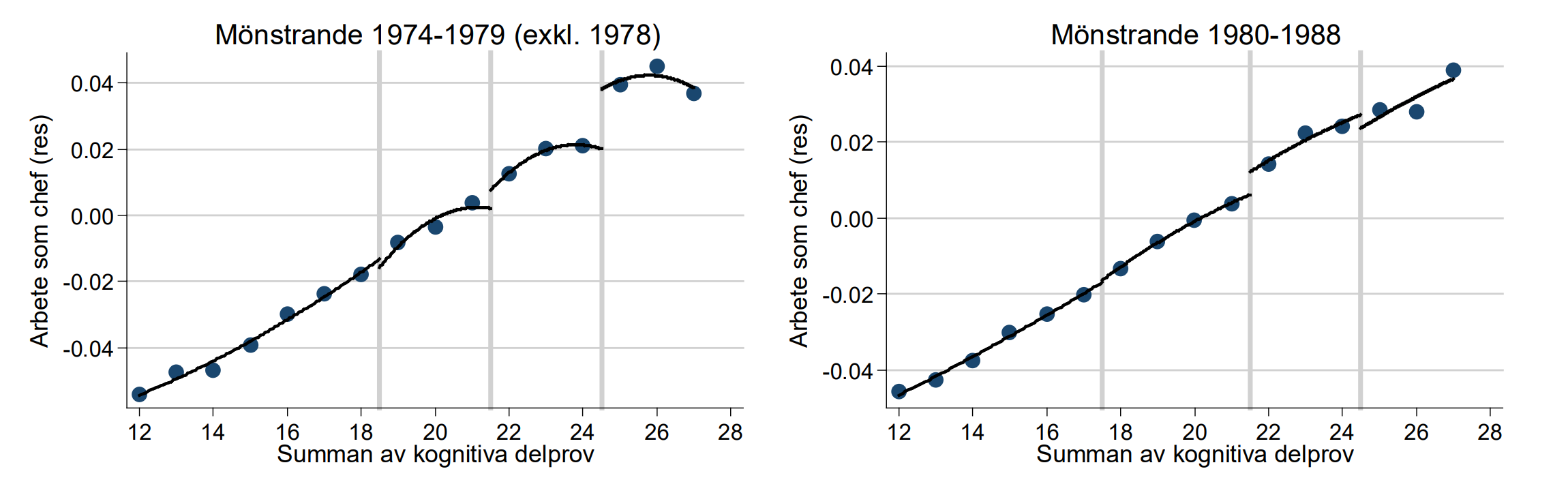
First look at the left panel showing the relationship in the 1970s. You can see a positive relationship: individuals who perform well on the tests have a much higher chance of later working as managers. Note the three vertical lines marking the cutoffs for squad leader, platoon leader and company commander. To qualify as a company commander you need, for example, at least 24.5 points on the tests. Right at this threshold the chance of becoming a manager rises sharply. An individual who scores 24.51 points — and thus qualifies for military leadership training — has a substantially greater chance of later becoming a manager in civilian life than a peer who scores 24.49.
4.5 The effects of immigration
We have now seen that education and experience matter for your income. But perhaps there are also things in your environment that affect how you fare in the labour market? One of the biggest social changes in recent decades is increased immigration. In Finland, for example, the number of immigrants has risen from 63,000 to 386,000 over the past 30 years. Maybe my success in the labour market depends on how many immigrants live where I live? But do more immigrants cause my wage to rise or fall?
Let’s try to crack that puzzle! To understand the challenge we can look at Sweden’s richest and poorest neighbourhoods: Höglandet in Bromma and Gamlegården in Kristianstad.

The share of immigrants is much higher in Gamlegården than in Bromma, so one possible explanation for the low earnings of native Swedes in Gamlegården is that far more immigrants live there than in Bromma. But how do you know it is the high immigration that makes wages so low in Gamlegården? Perhaps there are, for example, more students and poor pensioners moving to the depopulating suburb of Gamlestaden, where there are plenty of small empty flats. It’s probably no coincidence that so many immigrants live there while few end up in the multimillion‑euro villas of Bromma. Newly arrived migrants are not randomly spread across the country. Gamlestaden would likely have low incomes even without immigration. But how can we ever know?
David Card decided to investigate how immigration affected Americans. He exploited a so‑called natural experiment. In the summer of 1980 large numbers of Cubans fled on small boats, and most landed in Miami. Almost overnight the workforce in Miami grew by about 8 percent. The short video below summarises what happened to Miami’s unemployment when the Cubans arrived:
Mariel Boatlift was a mass migration of Cubans who left the port of Mariel, Cuba by boat for the US between 15 April and 31 October 1980. About 125,000 Cubans arrived in Miami in a short period. How did the US labour market respond to this large inflow of immigrants?
Here you can see in more detail what actually happened to unemployment according to Card. At the top of the table you can see what happened to unemployment in Miami over the period:
| Before | After | Change | Difference‑in‑differences | |
|---|---|---|---|---|
| Miami | 8.3% | 9.6% | +1.3 | -1.0 |
| Control cities | 10.3% | 12.6% | +2.3 |
As you can see, unemployment in Miami rose from 8.3% before the Mariel Boatlift to 9.6% after.
Many would interpret this as “immigration causes higher unemployment,” but how do we know what would have happened in Miami if the migrants had never arrived? In the early 1980s the whole US was suffering rising unemployment. That is why Card, cleverly, also checked what happened to unemployment in a set of other cities where the Cuban migrants did not arrive (just as in Chapter 1 we compared births in a Finnish municipality that did not introduce the baby bonus). As you can see, unemployment rose even more in these so‑called control cities. Card therefore concluded that the Cuban inflow to Miami did not increase unemployment among the native population. If anything, immigration led to lower unemployment.
4.6 Discrimination?
Or might your income depend on factors like gender and ethnicity? In Finland in 2023 the median annual income for people aged 18–64 born in Finland was €30,218, while the corresponding income for those born outside the EU was only €23,236. Discrimination is one possible explanation, but to be honest there are many other plausible causes.
Perhaps immigrants are, for example, younger or less educated than the native‑born population. Young and less educated people always earn less — regardless of whether they are immigrants or not. That could explain the wage gap between the groups. Or their lower incomes may reflect limited language skills, lack of networks and contacts, a concentration in lower‑paying sectors (such as service, restaurants and cleaning), less work experience, or weaker union support in wage negotiations. There are almost endless possible explanations. So how can we ever know whether discrimination truly exists in the labour market?
Claudia Goldin, who won the Nobel Prize in Economics in 2023, found a clever way to measure discrimination against women. In Goldin (2000) she examined audition outcomes for American symphony orchestras. When you apply for a job in a symphony orchestra you audition before a panel, much like on the TV show Idol. For a long time female musicians did very poorly in these auditions: orchestras hired almost only men. Critics pointed to gender discrimination, while orchestras claimed women simply weren’t good enough.
The researchers exploited a change in the recruitment procedure. Sometimes auditions were held behind a screen. Suddenly the jury could not tell whether the candidate was male or female. Suddenly only the performance itself determined the outcome. It’s almost like switching from Idol to The Voice. Behind the screen everything changed: women started succeeding just as often as men. This is clear evidence that gender discrimination was a major reason why female musicians had such difficulty getting jobs in American symphony orchestras.



Several studies have exploited similar “reforms.” Edin et al. (2006) analyse how employers choose which applicants to contact on the Swedish Public Employment Service’s online platform. Female applicants were 15% less likely to be contacted compared with a male applicant with identical qualifications. The site also allowed applicants to hide selected parts of their identity — and the researchers found — just like in the US symphony auditions of the 1980s — that women who did not reveal they were women performed as well as equivalently qualified men.

A tip is to draw inspiration from what others have done — and then do something of your own. Rooth et al. (2005), for example, studied how the September 11, 2001 attacks affected the labour‑market prospects of Muslims in Sweden. Several studies suggest the attacks changed attitudes toward immigrants; on 12 September fewer people were positive about immigration than on 10 September. But did this also make it harder for immigrants in Sweden to get jobs? The researchers therefore looked at how different immigrant groups’ chances of finding work changed before versus after 11 September 2001. The answer was that it became harder overall, but the same deterioration occurred for people born in Sweden. The potentially most exposed groups (the Middle East and Africa) did not experience larger declines in employment probability after 11 September than the Sweden‑born.
Turku has also been hit by terror. On 18 August 2017 ten people were stabbed at the Market Square in Turku. The attacker’s aim was to promote the ideology of the Islamic State (IS). Perhaps this attack made it harder for immigrants on the Finnish labour market? You can investigate this puzzle by, just like Rooth et al., looking in the data here at how unemployment among foreign‑born people evolved before and after the attack — and then comparing that development with what happened to unemployment among the Finland‑born. Only your imagination limits the questions you can explore.
4.7 Children and/or career?
Let’s finally return to pregnant Kaija Vilponen‑Liimatainen in Lestijärvi. How can we expect her income to be affected by becoming a mother?
Women with children earn less than women without children in almost every country. There are two possible explanations. The first is that having children causes lower earnings. The second is that there is something special about women who have children — that is, these women would have had low earnings even if they had not had children. So how can we get around this difficulty?
Lundborg et al. (2017) follow tens of thousands of Danish women who underwent IVF treatment (in vitro fertilisation) in the 1990s. This has the advantage that all potential parents in the sample clearly wanted a child. But IVF does not automatically result in a birth; only about one in three IVF attempts succeeds, and it seems impossible to know in advance why some attempts work and others don’t. It’s almost as if the stork arrives at random for some couples. So what happened to the earnings of the women who were lucky enough to have a child, and what happened to the earnings of the women who were unlucky? The answer is shown here:
| Year before IVF | Four years after IVF | Difference | Difference‑in‑differences | |
|---|---|---|---|---|
| Women who had a child | 243,012 | 211,525 | -32,387 | -28,842 |
| Women who did not have a child | 245,360 | 241,815 | -3,545 |
As you can see in the table above, annual earnings fell sharply for women whose IVF succeeded, whereas no comparable decline is seen among women whose IVF failed. Having a child appears to reduce annual income four years later by DKK 29,000 — roughly an 11–12% drop.
Bensnes et al. (2023) also follow IVF patients, but they track Norwegian couples over a much longer period (12 years). These researchers likewise find that children lead to large short‑term earnings losses for women: for example, annual incomes of those who gave birth were about 22% lower when the child was one year old (compared with incomes of women who remained childless). But in the longer run incomes recover. Twelve years after birth the “income penalty” for women who had children was only about 3%. Fathers’ incomes did not fall; on the contrary, fathers’ incomes rose by roughly 10% in the long run. Explain that if you can!
4.8 Are income inequalities fair?
In this chapter you learned how to research income differences — and you saw some factors that cause some people to get more money than others.
Is this fair? Economists find that hard to answer. What is fair or unfair is a normative question: your view of a fair distribution will almost certainly differ from mine — and it’s impossible to say which of us is “right.” Your opinion is as valid as mine.

An example of a normative statement is: “I think study grants should be raised to €700.” Some would support this: “it would get more people into higher education and that’s good for Finland” and “it would reduce unequal access to university.” Others would oppose it: “students already earn more than the rest of the population over their lifetimes” and “the money should instead be spent on children with cancer.” Who is right?
positive analysis is about how something is, normative analysis about how something ought to be.
Economists therefore usually focus on describing how things are. This is called positive analysis. A positive statement is either true or false: “The study grant is €279 per month” or “The capital of Spain is London.” Economists can only say how things are and explain how a given policy would affect society. It is then up to politicians and public opinion to decide whether to implement the proposal.
What do you think about inequality in society? Do you believe the market leads to unfairness? Is there too much cheap liquor and too little organic food? Is food too expensive and the study grant too low? In the next chapter we will see how politicians can intervene in markets using economic policy.
Exercises
Below are some cases where you can apply your knowledge in practice to analyse the labour market. Press Show Answers when you want the computer to grade your responses. Good luck!
Is two glasses of wine really healthy?
The claim “two glasses of wine a week work wonders for your health” is often heard in debates about alcohol.

- The fact that people who drink two glasses of wine a week are healthier than others does not necessarily mean that drinking two glasses causes better health. Explain why!
- As of 1 August 2025 mobile phones were banned in all Finnish comprehensive schools, see YLE. But are phones really harmful to learning? Researchers have proposed a randomised trial with a total ban, where the lottery determines which pupils lose their phones. Why would such a trial likely produce more credible conclusions than simply comparing pupils who use phones a lot with those who use them little?
- Young people who often drink Coca‑Cola Zero have worse health than those who rarely drink it. Yet randomised experiments, where chance assigns who drinks much or little Coca‑Cola Zero, show that this kind of soft drink does not cause worse health. Can you explain these seemingly contradictory findings?
- In your bachelor thesis you study the effects of alcohol. Which specific outcome would you investigate — i.e. how does alcohol affect what, exactly?
- Finland has 288 Alko stores and Sweden’s Systembolaget has 421 outlets. How could you use this variation to measure alcohol’s effects in your thesis? Take inspiration from David Card’s “proximity to school” trick.
- Sometimes there are large, sudden policy changes on alcohol. From 10 June 2024 Finland allowed the sale in grocery stores of drinks up to 8% ABV. A similar change occurred in Sweden on 1 October 1965 when “medium beer” was introduced in supermarkets. How could you use such reforms to measure alcohol’s effects? Take inspiration from David Card’s “Mariel Boatlift” trick.
- Suppose there are other differences between people who drink two glasses of wine a week and those who do not — and those differences affect health. Think stereotyping! Maybe high‑income thirty‑somethings uncork a bottle of Domaine Leroy Musigny Grand Cru on Friday nights? These people also enjoy other life circumstances that tend to produce good health — good finances, pleasant jobs, the ability to work from home, access to exercise — so perhaps it’s those factors, not the wine itself, that explain their good health.
- Think prejudicially: imagine a chaotic classroom where the teacher is incompetent and the pupils are troublemakers who smoke and play on their phones, versus Harvard, the world’s most prestigious institution. Is it really the phone that explains the poor results in the first classroom? Letting a lottery decide which classrooms ban phones would ensure, on average, that classrooms with and without phones look similar at baseline.
- Are there other differences — beyond soft‑drink consumption — between youths who drink 7 litres of Coca‑Cola every day and youths who drink much less? Maybe those other differences explain the poorer health of the heavy soda drinkers.
- Let your imagination run wild!
- Check whether the characteristic you’re interested in above is more common among people living near an Alko store.
- What happened in Sweden when beer suddenly became available in supermarkets? Do you see the same development in places that did not introduce the reform at the same time (for example Finland)?
Immigration and its effects
Here you can see the share of the population that was born in another country. The map shows the situation in 2024, but you can also change the time period by adjusting the slider below the map.
- The share of foreign‑born residents in Finland in 2024 was about . The corresponding figure in 1990 was .
- Which country in the world had the lowest share of foreign‑born residents in 2024? .
- Which country increased its immigrant share the most in percentage terms over 1990–2024 (in terms of foreign‑born population)? .
- Which country decreased its immigrant share the most in percentage terms over 1990–2024 (in terms of foreign‑born population)? .
- Explain, in your own words, how David Card used the Mariel Boatlift to study how immigration affects wages for people already living in the US.
- Researchers argue that immigrants from poor countries such as Cuba are substitutes for low‑skilled Americans but complements for high‑skilled Americans. What does that mean?
- Suppose immigrants from poor countries like Cuba are substitutes for low‑skilled Americans but complements for high‑skilled Americans. Why would immigration then lead to lower wages for low‑skilled Americans but higher wages for high‑skilled Americans (i.e. increased income inequality)?
- All social science students at Åbo Akademi must write a scientific paper at the end of their first year. You want to investigate whether increased immigration really leads to greater income inequality across countries. Your strategy is to make an Excel scatterplot showing immigration changes for each country over 1990–2024 (South Korea is a point far to the right, Cuba far to the left). On the Y‑axis you plot changes in the GINI coefficient for each country. You let the computer draw the best‑fit trend line. How should the trend line slope if immigrants are substitutes for low‑skilled workers but complements for high‑skilled workers?
- Explain, in your own words, how Claudia Goldin used data from US symphony orchestra hiring (auditions) to detect whether women faced discrimination in job recruitment.
- Play and explore the world by clicking Table, Map and Chart.
- You can sort by clicking the arrows when you are on Table.
- You can sort by clicking the arrows when you are on Table.
- You can sort by clicking the arrows when you are on Table.
- The method is called difference‑in‑differences. Can you summarise Card’s method and conclusions in two clear sentences for the exam? Try it now! Then read your two sentences and ask yourself: how would I grade this answer? Can I make it even clearer?
- Substitutes and complements were covered in Chapter 3.
- Imagine there were two types of Americans in Florida in 1980: high‑skilled and low‑skilled. Assume the Cubans who arrived on Miami’s shores were low‑skilled. The Cubans and low‑skilled Americans are substitutes: from employers’ perspective they are interchangeable, so the local supply of low‑skilled labour rises and wages for low‑skilled workers fall. High‑skilled Americans do not compete with the newcomers; instead the Cubans are a complement to them. According to comparative‑advantage logic, the Cubans make it possible for high‑skilled Americans to specialise more in their strengths — doctors, lawyers and executives no longer need to spend time on childcare, lawn mowing or other “simpler” tasks. They can go all in on their core tasks and become even more productive. As doctors, lawyers and executives become more productive, demand for them rises and their wages increase.
- If income inequality has risen most over the past 30 years in countries that received the most immigrants, the trend line should slope upwards.
- Can you summarise Goldin’s method and conclusions in two clear sentences for the exam? Try it now! Then read your two sentences and ask yourself: how would I grade this answer? Can I make it even clearer?
Why do immigrants earn less than natives?
Here is a table showing median income in 2025 (euros) for people aged 18–64 in several European countries. The first row thus shows Spain in 2025: the median income for those born in Spain was €25,068, while the corresponding figure for people in Spain born outside the EU was only €17,162. The foreign‑born in Spain therefore earned only 68.5% of the income of the Spain‑born. The data come from Eurostat.
| Country | Born in the country | Born outside the EU27 | Immigrants’ income (% of natives’) |
|---|---|---|---|
| Spain | 25 068 | 17 162 | 68,5 |
| Italy | 26 696 | 18 848 | 70,6 |
| Belgium | 37 670 | 26 676 | 70,8 |
| Sweden | 35 392 | 25 567 | 72,2 |
| Germany | 37 272 | 27 038 | 72,5 |
| France | 32 756 | 24 193 | 73,9 |
| Finland | 35 776 | 27 450 | 76,7 |
| Denmark | 43 898 | 35 152 | 80,1 |
| Greece | 14 345 | 11 672 | 81,4 |
| Estonia | 21 366 | 18 734 | 87,7 |
| Poland | 16 157 | 16 641 | 103,0 |
- Why do you think the income gap between native‑born people and those born outside the EU27 is smaller in Finland than in Sweden? Give at least three possible explanations.
- The incomes in the table are the median income. What does that mean?
- What happens to the median income if the highest earner in the country suddenly increases their income to €453 billion?
- What is the difference between percent and percentage points?
- “The study grant is €145” is an example of , whereas “The study grant should be increased by 10 percent” is an example of .
- Are different types of immigrants coming to Sweden than to Finland? Does Finland have better integration policy than Sweden? Is discrimination against immigrants greater in Sweden than in Finland?
- Read about mean vs median in the chapter.
- The median income is not affected at all.
- Percent refers to a part per hundred. If something rises from 50% to 55% it has increased by 5 percentage points, but that corresponds to a 10% increase relative to the original number (because 5/50 = 0.1 = 10%). Percentage points are therefore used to describe the difference between two percentages. If unemployment rises from 3% to 5% it has increased by 2 percentage points. Example: the Social Democrats in Finland received 17.7% in the 2019 parliamentary election and 19.9% in 2023 — an increase of 2.2 percentage points.
- If you want to learn more about Claudia Goldin’s research on women in the labour market, there is a popular‑science summary here.
- If you want to explore how inequality has evolved over time, you can investigate the World Inequality Database here. There you can, for example, see the share of national income going to the top 10% or the top 1% and how that has changed over the past 100 years.
- Tough day? If you need a pep talk from one of the US military’s senior officers, you can watch this. Maybe it offers some plausible explanations for why military leadership training raises wages in civilian life.