5 Policy interventions
(where you learn what happens when politicians step into the market)
In Chapter 3 you learned, among other things, that markets are efficient — at least under certain conditions. That means production and consumption, as if by miracle, end up being exactly what is best for society as a whole. An analogy for understanding efficiency is to think about the checkout queues at CityMarket.
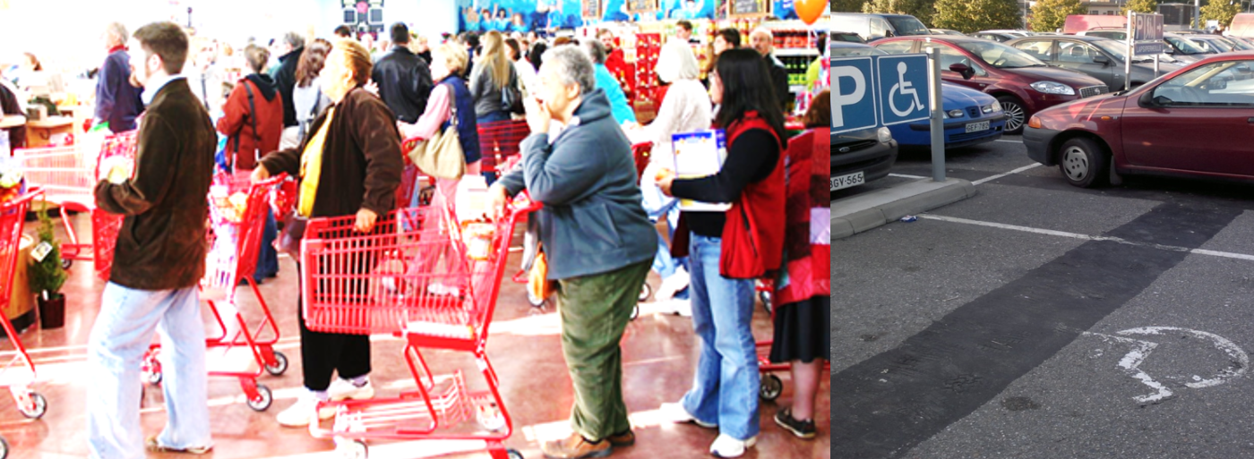
You’ve probably noticed that checkout lines in the supermarket are almost always equally long. That means there are no unexploited opportunities: most of us are rational enough to join the shortest queue because we want to get home as quickly as possible. When a new register opens it only takes a few seconds before the queues are equal again. So we do not waste time unnecessarily standing in line.
But not everything in life is about efficiency. Maybe you think one checkout should be reserved for customers over 90 so elderly people don’t have to wait, or that a few parking spaces near the entrance should be reserved for people with disabilities. That checkout and those parking spaces will often stand empty — an obvious waste — but it is a trade‑off you are willing to make to achieve fairness. Your values lead you to accept less efficiency for greater equity.
Similarly, we may dislike market outcomes. Perhaps you think there is too much drinking in Finland, that strawberries are too expensive, or that some groups earn too little. We will now see that politicians and policymakers have tools to steer markets in desired directions. In this chapter we will examine how those tools work and what effects they have on the economy.
5.1 Quotas limit the quantity
Imagine you are a municipal politician in Turku and you dislike the trade in strawberries at the Market Square. There is too much of it! You therefore decide to intervene in the market and limit the number of litres of strawberries that may be traded per day. In a fancier term this kind of “maximum quantity” is called a quota. Some markets you may want to shut down completely — it’s not obvious that everything should be traded merely because two parties voluntarily agree to exchange. Is it, for example, right to have markets for prostitution, surrogacy, crystal meth, kidneys, adoptive children, slaves or those tiny toys that kids can choke on? At other times you might want some trade to be allowed but not as much as in an unregulated market.
So how will a quota affect the market? Will strawberries become cheaper or more expensive and how will sellers and buyers be affected? The figure below shows what happens when you limit the quantity traded:
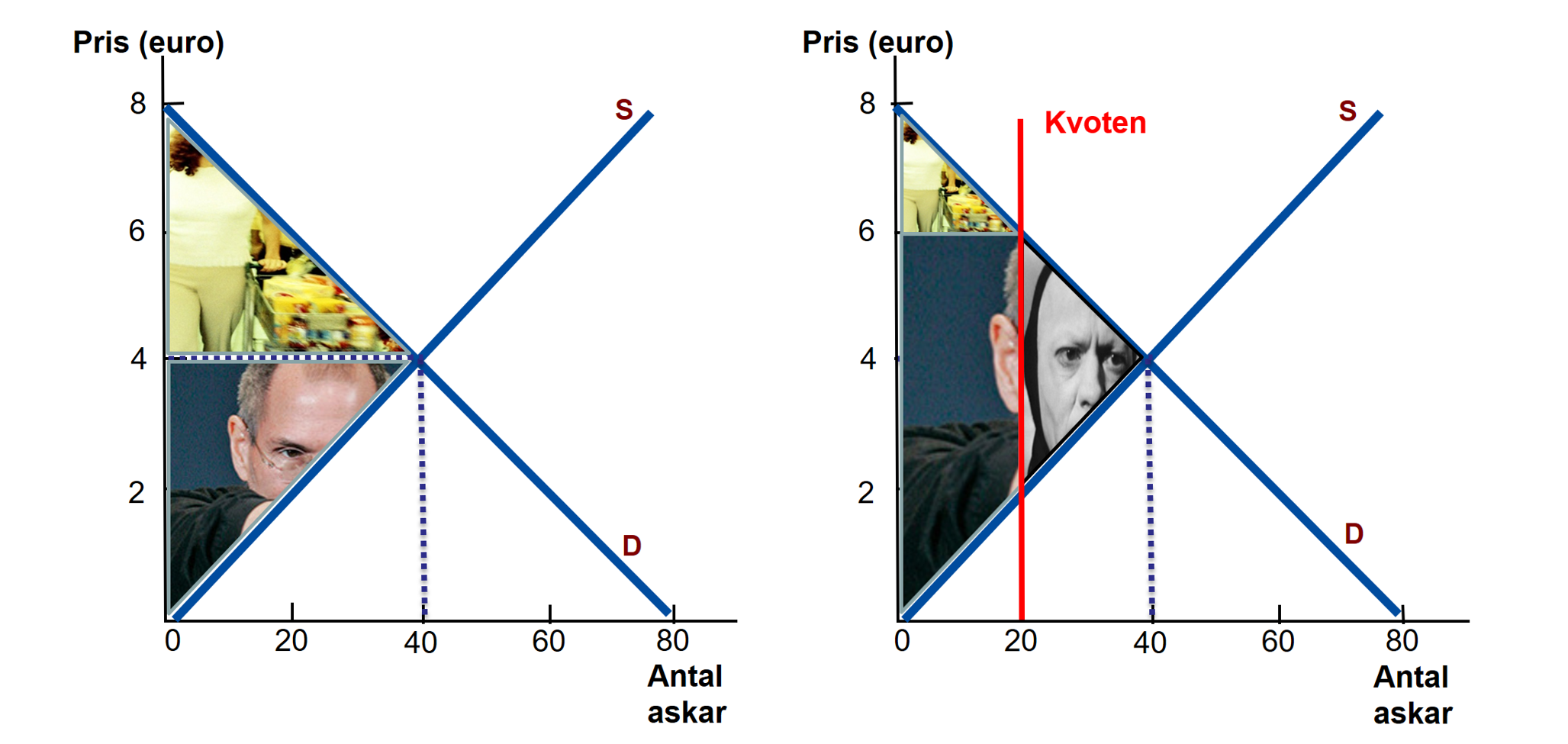
In the left-hand panel above the original situation is shown: 40 punnets of strawberries are sold at a price of €4 per punnet. The upper triangle (pictured as a shopper in the mall) represents consumer surplus — that is, how much more buyers collectively valued the strawberries than the price they actually paid. In this case CS = €80 (area of a triangle = base × height ÷ 2). The lower triangle (pictured as Apple founder Steve Jobs) shows producer surplus; here PS = €80, meaning sellers collectively received €80 more for the strawberries than the minimum they would have accepted.
Check: Do you know what CS and PS mean and can you calculate their sizes? If not, review Section 3.3 to refresh your knowledge.
In the right‑hand panel above you can see what happens when politicians limit trade to 20 punnets. The first thing you can observe is that trade becomes inefficiently small. How do you know that? Think at the margin: what would happen if one more unit were allowed to be sold? There are buyers willing to pay nearly €6 for the 21st punnet and sellers willing to accept just over €2 — yet that trade does not occur. Politicians have killed the possibility of that mutually beneficial exchange. The deadweight loss, illustrated in the figure by Death, is the value of all surplus that goes up in smoke when politicians eliminate part of the market.
The quota also makes strawberries more expensive. The demand curve shows what consumers are willing to pay for different quantities. If only 20 punnets may be sold, these punnets will go to the customers willing to pay at least €6 for a punnet. As a group consumers are therefore worse off under the quota: fewer and more expensive strawberries are bad news for people who come to the market to buy berries. The effect on sellers is theoretically ambiguous: they cannot sell as many punnets as before, which is bad, but they receive a higher price for the punnets they do sell, which is good. To determine whether the quota benefits or harms sellers as a group you therefore need to look at the data more closely.
In the app below you can experiment with quotas yourself. Play with the numbers and the computer will automatically produce an illustration and calculate exactly what happens. My advice is first to make sure you understand what is happening in the figure. Then learn to solve the problem yourself — in the exam you must be able to draw and calculate without aids. Practice until you master the technique.
The quota is the maximum quantity that may be sold.
Adjust the quota and see how price, quantity and deadweight loss are affected.
#| standalone: true
#| viewerHeight: 1440

# Lätt reviderad version av din ursprungliga app:
# - Behåller ursprunglig layout och funktionalitet
# - Bättre validering och användarfeedback
# - Korrigerade formler för KO/PÖ/Dödvikt (analytiska integraler)
# - Små robusthetsfixar och tydligare etiketter
if (!requireNamespace("shiny", quietly = TRUE)) install.packages("shiny")
if (!requireNamespace("ggplot2", quietly = TRUE)) install.packages("ggplot2")
if (!requireNamespace("plotly", quietly = TRUE)) install.packages("plotly")

library(shiny)
library(ggplot2)
library(plotly)

ui <- fluidPage(
  fluidRow(
    column(4,
      wellPanel(
        numericInput("supply_intercept", "Ange interceptet för utbudskurvan:", 10),
        numericInput("supply_slope", "Ange lutningen för utbudskurvan (positiv):", 0.5, min = 1e-6),
        numericInput("demand_intercept", "Ange interceptet för efterfrågekurvan:", 30),
        numericInput("demand_slope", "Ange lutningen för efterfrågekurvan (negativ):", -0.5, max = -1e-6),
        numericInput("x_max", "X-axelns maxvärde i figuren:", value = 50, min = 1),
        numericInput("y_max", "Y-axelns maxvärde i figuren:", value = 40, min = 1),
        # För att ange "ingen kvot" kan användaren lämna fältet tomt eller ange NA.
        # NumericInput i Shiny kan visa NA om value = NA initialt; vi sätter initialt NA.
        numericInput("quota", "Ange kvot (maximal mängd) eller lämna tomt för ingen kvot:", value = NA),
        actionButton("update", "Uppdatera figuren och beräkningarna",
                     style = "color: white; background-color: #007bff; padding: 6px 12px; border: 2px solid #007bff; font-size: 14px;"),
        br(),
        tags$h5("Användarguide: Fyll i parametrarna ovan och klicka på 'Uppdatera figuren och beräkningarna'."),
        tags$small("Obs: Utbudskurvan måste ha positiv lutning och efterfrågekurvan negativ.")
      )
    ),
    column(8,
      plotlyOutput("demandSupplyPlot"),
      br(),
      verbatimTextOutput("quotaEffect"),
      verbatimTextOutput("inverseFunctions")
    )
  )
)

server <- function(input, output, session) {

  # Håller validerade värden som bara uppdateras när användaren klickar 'update'
  validatedInput <- reactiveValues(
    supply_intercept = 10,
    supply_slope = 0.5,
    demand_intercept = 30,
    demand_slope = -0.5,
    quota = NA
  )

  observeEvent(input$update, {
    # Läs in råa värden
    si <- input$supply_intercept
    ss <- input$supply_slope
    di <- input$demand_intercept
    ds <- input$demand_slope
    q  <- input$quota

    # Grundläggande validering
    if (any(is.na(c(si, ss, di, ds)))) {
      showNotification("Ogiltig inmatning: Ange numeriska värden för alla kurvparametrar.", type = "error")
      return()
    }
    if (!is.numeric(ss) || ss <= 0) {
      showNotification("Utbuds-lutningen måste vara ett positivt tal.", type = "error")
      return()
    }
    if (!is.numeric(ds) || ds >= 0) {
      showNotification("Efterfråge-lutningen måste vara ett negativt tal.", type = "error")
      return()
    }
    if (!is.na(q) && (!is.numeric(q) || q < 0)) {
      showNotification("Kvoten måste vara ett icke-negativt tal eller lämnas tom.", type = "error")
      return()
    }

    # Spara validerade värden
    validatedInput$supply_intercept <- si
    validatedInput$supply_slope     <- ss
    validatedInput$demand_intercept <- di
    validatedInput$demand_slope     <- ds
    validatedInput$quota            <- ifelse(is.na(q), NA, q)
    showNotification("Parametrar uppdaterade.", type = "message")
  })

  # Hjälpfunktioner
  supply_at <- function(q, si, ss) si + ss * q
  demand_at <- function(q, di, ds) di + ds * q

  equilibrium <- reactive({
    si <- validatedInput$supply_intercept
    ss <- validatedInput$supply_slope
    di <- validatedInput$demand_intercept
    ds <- validatedInput$demand_slope

    # Om lutningarna lika -> ingen unik jämvikt
    if (abs(ss - ds) < .Machine$double.eps^0.5) return(list(eq_x = NA, eq_y = NA))
    eq_x <- (di - si) / (ss - ds)
    eq_y <- supply_at(eq_x, si, ss)
    if (is.na(eq_x) || is.na(eq_y) || eq_x < 0 || eq_y < 0) return(list(eq_x = NA, eq_y = NA))
    list(eq_x = eq_x, eq_y = eq_y)
  })

  # Korrekt beräkning av kvoteffekt (KO, PO, pris vid kvot) med analytiska formler
  quota_effect <- reactive({
    q <- validatedInput$quota
    eq <- equilibrium()
    si <- validatedInput$supply_intercept
    ss <- validatedInput$supply_slope
    di <- validatedInput$demand_intercept
    ds <- validatedInput$demand_slope

    # Om ingen kvot eller ingen giltig jämvikt eller kvoten inte binder -> NULL
    if (is.na(q) || is.na(eq$eq_x) || q >= eq$eq_x) return(NULL)

    # Pris som följer av efterfrågekurvan vid kvoten
    quota_price <- demand_at(q, di, ds)

    # Producentöverskott vid kvot (area mellan pris och utbudskurva, 0..q)
    # PO_q = q * P_q - integral_0^q (si + ss * x) dx
    #       = q * P_q - (si * q + 0.5 * ss * q^2)
    quota_PO <- round(q * quota_price - (si * q + 0.5 * ss * q^2), 2)

    # Konsumentöverskott vid kvot (triangle mellan efterfrågan och pris P_q, 0..q)
    # KO_q = 0.5 * q * (P_max - P_q) där P_max = di (pris vid Q=0 för linjär efterfrågan)
    quota_KO <- round(0.5 * q * (di - quota_price), 2)

    list(quota_price = round(quota_price, 2), KO = quota_KO, PO = quota_PO, quota = q)
  })


  output$demandSupplyPlot <- renderPlotly({
    # Säkerställ att användaren har uppdaterat parametrar åtminstone en gång
    req(validatedInput$supply_slope, validatedInput$demand_slope)

    si <- validatedInput$supply_intercept
    ss <- validatedInput$supply_slope
    di <- validatedInput$demand_intercept
    ds <- validatedInput$demand_slope
    x_max <- input$x_max
    y_max <- input$y_max
    q <- validatedInput$quota

    # Mer validering för axelintervall
    if (any(is.na(c(si, ss, di, ds, x_max, y_max)))) {
      showNotification("Ogiltig inmatning för plotparametrar.", type = "error")
      return(NULL)
    }

    x <- seq(0, x_max, length.out = 200)
    y_supply <- supply_at(x, si, ss)
    y_demand <- demand_at(x, di, ds)

    eq <- equilibrium()
    data <- data.frame(x = x, y_supply = y_supply, y_demand = y_demand)
    data <- data[data$y_demand >= 0 | data$y_supply >= 0, ] # visa relevanta delar

    # Enkel färgblindvänlig palett
    p <- ggplot(data, aes(x)) +
      geom_line(aes(y = y_supply, color = "Utbud"), size = 1) +
      geom_line(aes(y = y_demand, color = "Efterfrågan"), size = 1) +
      labs(x = "Mängd (Q)", y = "Pris (P)") +
      theme_minimal() +
      scale_color_manual(name = "Kurvor:", values = c("Utbud" = "#1b9e77", "Efterfrågan" = "#d95f02")) +
      theme(legend.title = element_blank()) +
      coord_cartesian(ylim = c(0, y_max), xlim = c(0, x_max)) +
      geom_hline(yintercept = 0, color = "black", size = 0.5) +
      geom_vline(xintercept = 0, color = "black", size = 0.5)

    # Visa jämvikt om giltig
    if (!is.na(eq$eq_x) && !is.na(eq$eq_y)) {
      p <- p +
        geom_point(aes(x = eq$eq_x, y = eq$eq_y), color = "purple", size = 3) +
        geom_segment(aes(x = eq$eq_x, xend = eq$eq_x, y = 0, yend = eq$eq_y), linetype = "dashed", color = "purple") +
        geom_segment(aes(x = 0, xend = eq$eq_x, y = eq$eq_y, yend = eq$eq_y), linetype = "dashed", color = "purple")

      # Om ingen kvot anges, visa KO och PO vid jämvikt
      if (is.na(q)) {
        # KO: area mellan demand och eq$eq_y från 0..eq_x
        p <- p +
          geom_ribbon(data = subset(data, x <= eq$eq_x), aes(ymin = eq$eq_y, ymax = y_demand), fill = "#a6cee3", alpha = 0.6) +
          geom_ribbon(data = subset(data, x <= eq$eq_x), aes(ymin = y_supply, ymax = eq$eq_y), fill = "#fdbf6f", alpha = 0.6)
      }
    }

    # Om kvot anges och den binder
    quotaInfo <- quota_effect()
    if (!is.null(quotaInfo)) {
      qval <- quotaInfo$quota
      Pq <- quotaInfo$quota_price

      # Konsumentöverskott & Producentöverskott upp till kvot
      p <- p +
        geom_ribbon(data = subset(data, x <= qval), aes(ymin = Pq, ymax = y_demand), fill = "#a6cee3", alpha = 0.6) +
        geom_ribbon(data = subset(data, x <= qval), aes(ymin = y_supply, ymax = Pq), fill = "#fdbf6f", alpha = 0.6)

      # Dödvikt: område mellan q och eq$eq_x
      if (!is.na(eq$eq_x) && qval < eq$eq_x) {
        dq <- seq(qval, eq$eq_x, length.out = 100)
        df_dw <- data.frame(x = dq,
                            ymin = supply_at(dq, si, ss),
                            ymax = demand_at(dq, di, ds))
        p <- p + geom_ribbon(data = df_dw, aes(x = x, ymin = ymin, ymax = ymax), fill = "grey40", alpha = 0.4)
      }

      p <- p + geom_vline(xintercept = qval, linetype = "dashed", color = "darkgreen")
    }

    ggplotly(p)
  })

  output$inverseFunctions <- renderText({
    si <- validatedInput$supply_intercept
    ss <- validatedInput$supply_slope
    di <- validatedInput$demand_intercept
    ds <- validatedInput$demand_slope

    supply_inverse <- if (ss != 0) {
      paste0("Q = (P - ", si, ") / ", ss)
    } else {
      "Utbudslinjen kan inte inverteras (lutning = 0)."
    }

    demand_inverse <- if (ds != 0) {
      paste0("Q = (P - ", di, ") / ", ds)
    } else {
      "Efterfrågelinjen kan inte inverteras (lutning = 0)."
    }

    paste("Utbud: ", supply_inverse, "\nEfterfrågan: ", demand_inverse)
  })

  output$quotaEffect <- renderText({
    eq <- equilibrium()
    quotaEffect <- quota_effect()

    originalEquilibriumText <- if (is.na(eq$eq_x) || is.na(eq$eq_y)) {
      "Jämvikt: Ingen skärningspunkt vid positiva värden"
    } else {
      price <- round(eq$eq_y, 2)
      quantity <- round(eq$eq_x, 2)
      # Konsumentöverskott och producentöverskott vid jämvikt - konsekventa formler
      KO <- round(0.5 * quantity * (validatedInput$demand_intercept - price), 2)
      PO <- round(quantity * price - (validatedInput$supply_intercept * quantity + 0.5 * validatedInput$supply_slope * quantity^2), 2)
      paste("Jämvikt:", "\nPris:", price, "\nMängd:", quantity, "\nKonsumentöverskott (KÖ):", KO, "\nProducentöverskott (PÖ):", PO)
    }

    if (is.null(quotaEffect)) {
      paste(originalEquilibriumText, "\n\nIngen kvot är angiven eller kvoten påverkar ej jämvikten.")
    } else {
      # Dödvikt = (KO_eq + PO_eq) - (KO_q + PO_q)
      # Återberäkna KO_eq och PO_eq med samma formler som ovan
      if (is.na(eq$eq_x) || is.na(eq$eq_y)) {
        DÖ <- NA
      } else {
        price <- round(eq$eq_y, 2)
        quantity <- round(eq$eq_x, 2)
        KO_eq <- 0.5 * quantity * (validatedInput$demand_intercept - price)
        PO_eq <- quantity * price - (validatedInput$supply_intercept * quantity + 0.5 * validatedInput$supply_slope * quantity^2)
        DÖ <- round((KO_eq + PO_eq) - (quotaEffect$KO + quotaEffect$PO), 2)
      }

      paste(originalEquilibriumText,
            "\n\nMed kvot:",
            "\nPris:", quotaEffect$quota_price,
            "\nMängd:", quotaEffect$quota,
            "\nKonsumentöverskott (KÖ):", quotaEffect$KO,
            "\nProducentöverskott (PÖ):", quotaEffect$PO,
            "\nDödviktsförlust (DÖ):", ifelse(is.na(DÖ), "NA", DÖ))
    }
  })
}

shinyApp(ui = ui, server = server)
5.2 Price ceiling lowers the price
There is now a change of power in the municipality. Your colleague takes over. Her first action is to remove the restrictions on strawberry trade. However, she thinks the price of €4 per punnet of strawberries is far too high.
“Even poor ÅA students must be able to afford strawberries!” she thunders in the local paper.
To push prices down she therefore introduces a price ceiling of €2 per punnet. This means strawberries may not be sold for more than €2. You can think of a price ceiling as a roof you bang your head on — an upper limit. The figure below shows how the price ceiling affects the market:
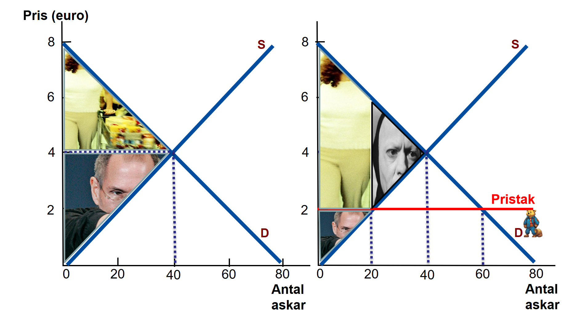
Remember that the supply curve shows how much producers are willing to sell at different prices. With a price ceiling of €2 producers are only willing to sell 20 litres of strawberries. You cannot force them to sell more than that. Trade in strawberries is therefore inefficiently small again. The price ceiling prevents some exchanges that would have benefited both buyers and sellers. The deadweight loss shown in the figure indicates that total welfare (the sum of CS and PS) falls.
The figure also shows how different groups are affected by the price ceiling. For example, producer surplus falls when the ceiling is introduced. That sellers lose is unsurprising: lower price and lower sales are clearly bad news for them. For buyers the effect is theoretically ambiguous: strawberries become cheaper (good!), but they cannot buy as many as before (bad!). Theory therefore cannot tell us for certain whether the ceiling helps consumers. If you want to be picky, the consumer surplus shown in the figure is very likely an overestimate of true consumer surplus. Do you see why? Think this through: at price €2 consumers would like 60 litres, but only 20 are sold. How should we choose which customers get the 20 punnets? In a normal market it is price that decides who gets what, but here politicians have taken market forces out of action. In my illustration of CS I assumed the punnets go to exactly those consumers who value them most — i.e. Jenny (willing to pay €8) gets berries while allergic Anton (willing to pay €2) does not (see Figure 3.3). In practice there is nothing to guarantee this: the 20 punnets could just as well end up with Anton and similar low‑valuation buyers.
Example: rent controls. Suppose the state caps rents at €300/month. Low rents are nice, but our analysis also shows that the cap reduces the number of apartments offered for rent. The intervention “kills” many housing transactions that would have benefited both tenants and landlords. People’s willingness to trade is strong — and there is a real risk that black markets will appear where parties trade in secret. If you fail to get an apartment on the cheap legal market you might find someone on the black market willing to rent it to you for €500. In an exercise at the end of the chapter you will study how such price ceilings affected Sweden’s housing market.
Below is an app that helps you analyse the effects of a price ceiling in more detail.
#| standalone: true
#| viewerHeight: 1470

if (!requireNamespace("shiny", quietly = TRUE)) install.packages("shiny")
if (!requireNamespace("ggplot2", quietly = TRUE)) install.packages("ggplot2")
if (!requireNamespace("plotly", quietly = TRUE)) install.packages("plotly")

library(shiny)
library(ggplot2)
library(plotly)

ui <- fluidPage(
  fluidRow(
    column(4,
      wellPanel(
        numericInput("supply_intercept", "Ange interceptet för utbudskurvan:", 10),
        numericInput("supply_slope", "Ange lutningen för utbudskurvan (positiv):", 0.5, min = 1e-6),
        numericInput("demand_intercept", "Ange interceptet för efterfrågekurvan:", 30),
        numericInput("demand_slope", "Ange lutningen för efterfrågekurvan (negativ):", -0.5, max = -1e-6),
        numericInput("x_max", "X-axelns maxvärde i figuren:", value = 50, min = 1),
        numericInput("y_max", "Y-axelns maxvärde i figuren:", value = 40, min = 1),
        numericInput("price_ceiling", "Ange pristak (lämna tomt för inget):", value = NA),
        actionButton("update", "Uppdatera figuren och beräkningarna",
                     style = "color: white; background-color: #007bff; padding: 6px 12px; border: 2px solid #007bff; font-size: 14px;"),
        br(),
        tags$h5("Användarguide: Fyll i parametrarna ovan och klicka på 'Uppdatera'."),
        tags$small("Obs: Utbudskurvan måste ha positiv lutning och efterfrågekurvan negativ.")
      )
    ),
    column(8,
      plotlyOutput("demandSupplyPlot"),
      br(),
      verbatimTextOutput("priceCeilingEffect"),
      verbatimTextOutput("inverseFunctions")
    )
  )
)

server <- function(input, output, session) {

  validatedInput <- reactiveValues(
    supply_intercept = 10,
    supply_slope = 0.5,
    demand_intercept = 30,
    demand_slope = -0.5,
    price_ceiling = NA
  )

  observeEvent(input$update, {
    si <- input$supply_intercept
    ss <- input$supply_slope
    di <- input$demand_intercept
    ds <- input$demand_slope
    pc <- input$price_ceiling

    if (any(is.na(c(si, ss, di, ds)))) {
      showNotification("Ogiltig inmatning: Ange numeriska värden för alla kurvparametrar.", type = "error")
      return()
    }
    if (!is.numeric(ss) || ss <= 0) {
      showNotification("Utbuds-lutningen måste vara ett positivt tal.", type = "error")
      return()
    }
    if (!is.numeric(ds) || ds >= 0) {
      showNotification("Efterfråge-lutningen måste vara ett negativt tal.", type = "error")
      return()
    }
    if (!is.na(pc) && (!is.numeric(pc) || pc < 0)) {
      showNotification("Pristaket måste vara ett icke-negativt tal eller lämnas tom.", type = "error")
      return()
    }

    validatedInput$supply_intercept <- si
    validatedInput$supply_slope     <- ss
    validatedInput$demand_intercept <- di
    validatedInput$demand_slope     <- ds
    validatedInput$price_ceiling    <- ifelse(is.na(pc), NA, pc)
    showNotification("Parametrar uppdaterade.", type = "message")
  })

  supply_at <- function(q, si, ss) si + ss * q
  demand_at <- function(q, di, ds) di + ds * q

  equilibrium <- reactive({
    si <- validatedInput$supply_intercept
    ss <- validatedInput$supply_slope
    di <- validatedInput$demand_intercept
    ds <- validatedInput$demand_slope

    if (abs(ss - ds) < .Machine$double.eps^0.5) return(list(eq_x = NA, eq_y = NA))
    eq_x <- (di - si) / (ss - ds)
    eq_y <- supply_at(eq_x, si, ss)
    if (is.na(eq_x) || is.na(eq_y) || eq_x < 0 || eq_y < 0) return(list(eq_x = NA, eq_y = NA))
    list(eq_x = eq_x, eq_y = eq_y)
  })

  price_ceiling_effect <- reactive({
    pc <- validatedInput$price_ceiling
    eq <- equilibrium()
    si <- validatedInput$supply_intercept
    ss <- validatedInput$supply_slope
    di <- validatedInput$demand_intercept
    ds <- validatedInput$demand_slope

    if (is.na(pc) || is.na(eq$eq_y) || pc >= eq$eq_y) return(NULL)

    q_supply <- (pc - si) / ss
    q_demand <- (pc - di) / ds

    q_supply <- round(max(0, q_supply), 8)
    q_demand <- round(max(0, q_demand), 8)

    excess_demand <- round(max(0, q_demand - q_supply), 2)

    list(quantity_supplied = round(q_supply, 2),
         quantity_demanded = round(q_demand, 2),
         excess_demand = excess_demand,
         price_ceiling = pc)
  })

  output$demandSupplyPlot <- renderPlotly({
    req(validatedInput$supply_slope, validatedInput$demand_slope)

    si <- validatedInput$supply_intercept
    ss <- validatedInput$supply_slope
    di <- validatedInput$demand_intercept
    ds <- validatedInput$demand_slope
    x_max <- input$x_max
    y_max <- input$y_max
    pc <- validatedInput$price_ceiling

    if (any(is.na(c(si, ss, di, ds, x_max, y_max)))) {
      showNotification("Ogiltig inmatning för plotparametrar.", type = "error")
      return(NULL)
    }

    x <- seq(0, x_max, length.out = 200)
    y_supply <- supply_at(x, si, ss)
    y_demand <- demand_at(x, di, ds)

    eq <- equilibrium()
    data <- data.frame(x = x, y_supply = y_supply, y_demand = y_demand)
    data <- data[data$y_demand >= 0 | data$y_supply >= 0, ]

    p <- ggplot(data, aes(x)) +
      geom_line(aes(y = y_supply, color = "Utbud"), size = 1) +
      geom_line(aes(y = y_demand, color = "Efterfrågan"), size = 1) +
      labs(x = "Mängd (Q)", y = "Pris (P)", color = NULL) +
      theme_minimal(base_size = 10) +
      scale_color_manual(name = "Kurvor:", values = c("Utbud" = "#1b9e77", "Efterfrågan" = "#d95f02")) +
      theme(legend.title = element_blank(),
            legend.text  = element_text(size = 9),           # legendens textstorlek
            legend.key.size = unit(16, "pt")                 # storlek på legendboxarna
  ) +


      coord_cartesian(ylim = c(0, y_max), xlim = c(0, x_max)) +
      geom_hline(yintercept = 0, color = "black", size = 0.5) +
      geom_vline(xintercept = 0, color = "black", size = 0.5)

    if (!is.na(eq$eq_x) && !is.na(eq$eq_y)) {
      p <- p +
        geom_point(aes(x = eq$eq_x, y = eq$eq_y), color = "purple", size = 3) +
        geom_segment(aes(x = eq$eq_x, xend = eq$eq_x, y = 0, yend = eq$eq_y), linetype = "dashed", color = "purple") +
        geom_segment(aes(x = 0, xend = eq$eq_x, y = eq$eq_y, yend = eq$eq_y), linetype = "dashed", color = "purple")
    }

    pc_info <- price_ceiling_effect()
    if (!is.null(pc_info)) {
      qs <- pc_info$quantity_supplied
      qd <- pc_info$quantity_demanded
      pc_val <- pc_info$price_ceiling

      p <- p + geom_hline(yintercept = pc_val, linetype = "solid", color = "darkgreen", size = 1)

      if (qs > 0) {
        p <- p +
          geom_ribbon(data = subset(data, x <= qs), aes(ymin = y_supply, ymax = pc_val), fill = "#fdbf6f", alpha = 0.6) +
          geom_ribbon(data = subset(data, x <= qs), aes(ymin = pc_val, ymax = y_demand), fill = "#a6cee3", alpha = 0.6)
      }

      if (!is.na(eq$eq_x) && qs < eq$eq_x) {
        dq <- seq(qs, eq$eq_x, length.out = 100)
        df_dw <- data.frame(x = dq,
                            ymin = supply_at(dq, si, ss),
                            ymax = demand_at(dq, di, ds))
        p <- p + geom_ribbon(data = df_dw, aes(x = x, ymin = ymin, ymax = ymax), fill = "grey40", alpha = 0.4)
      }
    }

    ggplotly(p) %>%
      layout(
        font = list(size = 14, family = "Arial"),
        legend = list(bgcolor = "rgba(255,255,255,0.9)", x = 0.85, y = 0.85, xanchor = "right")
      )
  })

  output$inverseFunctions <- renderText({
    si <- validatedInput$supply_intercept
    ss <- validatedInput$supply_slope
    di <- validatedInput$demand_intercept
    ds <- validatedInput$demand_slope

    supply_inverse <- if (ss != 0) {
      paste0("Q = (P - ", si, ") / ", ss)
    } else {
      "Utbudslinjen kan inte inverteras (lutning = 0)."
    }

    demand_inverse <- if (ds != 0) {
      paste0("Q = (P - ", di, ") / ", ds)
    } else {
      "Efterfrågelinjen kan inte inverteras (lutning = 0)."
    }

    paste("Utbud: ", supply_inverse, "\nEfterfrågan: ", demand_inverse)
  })

  output$priceCeilingEffect <- renderText({
    eq <- equilibrium()
    pcEffect <- price_ceiling_effect()

    originalEquilibriumText <- if (is.na(eq$eq_x) || is.na(eq$eq_y)) {
      "Jämvikt: Ingen skärningspunkt vid positiva värden"
    } else {
      price <- round(eq$eq_y, 2)
      quantity <- round(eq$eq_x, 2)
      KO <- round(0.5 * quantity * (validatedInput$demand_intercept - price), 2)
      PO <- round(quantity * price - (validatedInput$supply_intercept * quantity + 0.5 * validatedInput$supply_slope * quantity^2), 2)
      paste("Jämvikt:", "\nPris:", price, "\nMängd:", quantity, "\nKonsumentöverskott (KÖ):", KO, "\nProducentöverskott (PÖ):", PO)
    }

    if (is.null(pcEffect)) {
      paste(originalEquilibriumText, "\n\nInget pristak är angivet eller pristaket påverkar ej jämvikten.")
    } else {
      pc <- pcEffect$price_ceiling
      qs <- pcEffect$quantity_supplied
      qd <- pcEffect$quantity_demanded
      excess <- pcEffect$excess_demand

      demand_price_at_qs <- demand_at(qs, validatedInput$demand_intercept, validatedInput$demand_slope)
      upper_triangle_KO <- 0.5 * qs * (validatedInput$demand_intercept - demand_price_at_qs)
      rectangle_KO <- qs * (demand_price_at_qs - pc)
      total_KO <- round(upper_triangle_KO + rectangle_KO, 2)

      PO <- round(qs * pc - (validatedInput$supply_intercept * qs + 0.5 * validatedInput$supply_slope * qs^2), 2)

      if (is.na(eq$eq_x) || is.na(eq$eq_y)) {
        deadweight_loss <- NA
      } else {
        orig_KO <- 0.5 * eq$eq_x * (validatedInput$demand_intercept - eq$eq_y)
        orig_PO <- eq$eq_x * eq$eq_y - (validatedInput$supply_intercept * eq$eq_x + 0.5 * validatedInput$supply_slope * eq$eq_x^2)
        deadweight_loss <- round((orig_KO + orig_PO) - (total_KO + PO), 2)
      }

      paste(originalEquilibriumText,
            "\n\nMed pristak:",
            "\nMängd som erbjuds vid pristaket:", qs,
            "\nMängd som efterfrågas vid pristaket:", qd,
            "\nÖverskottsefterfrågan:", excess,
            "\nKonsumentöverskott (KÖ):", total_KO,
            "\nProducentöverskott (PÖ):", PO,
            "\nDödviktsförlust (DÖ):", ifelse(is.na(deadweight_loss), "NA", deadweight_loss),
            "\n\nPristak:", pc)
    }
  })
}

shinyApp(ui = ui, server = server)
5.3 Price floor raises the price
Other politicians think the strawberries are too cheap.
“Even poor growers must be able to make a living from strawberries!” they thunder in the local paper.
They therefore introduce a price floor of €6 per punnet. A mnemonic: a floor is something you stand on — a lower bound. The figure below shows how the price floor affects the market:
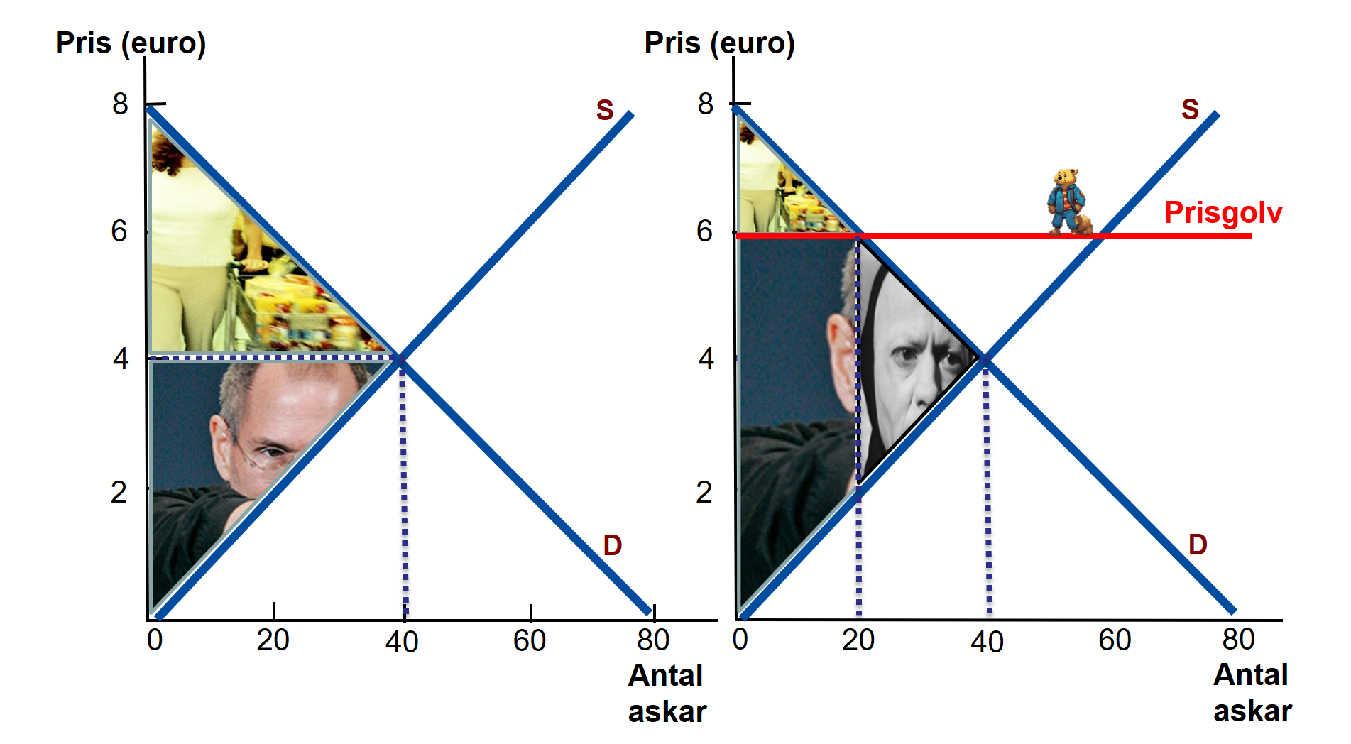
Imagine the price of strawberries rises to €6. How does that affect market participants? Buyers will not want to buy as much as before; the demand curve above shows they would buy only 20 litres at this high price. You cannot force consumers to buy more than they want, so trade becomes inefficiently small under the price floor. The deadweight loss in the figure shows the price floor reduces total welfare (the sum of CS and PS).
The figure also shows how the floor affects different groups. Consumer surplus falls when the floor is introduced — unsurprising: higher prices and less trade are bad news for buyers. For sellers the effect is theoretically ambiguous: they receive a higher price (good!) but cannot sell as much as before (bad!). Another problem arises: at €6 producers would be willing to supply 60 litres, so which sellers will actually sell the 20 litres that buyers purchase? In my diagram I assumed that the 20 punnets are miraculously sold by low‑cost producers like Pia (see Figure 3.3). In reality there is no guarantee of that; the punnets could just as well be sold by producers who would only supply at €5 or €6. The producer surplus shown is therefore likely an overestimate of how well producers are actually off under the price floor.
Example: minimum wages. Price floors appear in labour markets as minimum wages. Suppose the state legislates that no one may earn less than €3,000 per month. A high wage is attractive, but our analysis also shows the reform reduces employment: the intervention “kills” some jobs that would have benefited both buyers and sellers of labour. There is a real risk that black markets will arise where parties meet secretly to transact. If you cannot hire a worker on the expensive legal market you might find someone on the black market willing to work for €2,000. In an exercise at the end of the chapter you will study how minimum wages affect the labour market.
Below is an app to help you analyse the effects of a price floor in more detail.
#| standalone: true
#| viewerHeight: 1470

# Reviderad och robust version av prisgolvs-appen.
# - Samma layout och stil som pristak- och kvot-apparna
# - Tydligare validering och användarfeedback
# - Konsekventa analytiska formler för KO/PÖ/DÖ
# - Hantering av kantfall (lutning = 0, negativa värden, osv.)

if (!requireNamespace("shiny", quietly = TRUE)) install.packages("shiny")
if (!requireNamespace("ggplot2", quietly = TRUE)) install.packages("ggplot2")
if (!requireNamespace("plotly", quietly = TRUE)) install.packages("plotly")

library(shiny)
library(ggplot2)
library(plotly)

ui <- fluidPage(
  fluidRow(
    column(4,
      wellPanel(
        numericInput("supply_intercept", "Ange interceptet för utbudskurvan:", 10),
        numericInput("supply_slope", "Ange lutningen för utbudskurvan (positiv):", 0.5, min = 1e-6),
        numericInput("demand_intercept", "Ange interceptet för efterfrågekurvan:", 30),
        numericInput("demand_slope", "Ange lutningen för efterfrågekurvan (negativ):", -0.5, max = -1e-6),
        numericInput("x_max", "X-axelns maxvärde i figuren:", value = 50, min = 1),
        numericInput("y_max", "Y-axelns maxvärde i figuren:", value = 40, min = 1),
        numericInput("price_floor", "Ange prisgolv (lämna tomt för inget):", value = NA),
        actionButton("update", "Uppdatera figuren och beräkningarna",
                     style = "color: white; background-color: #007bff; padding: 6px 12px; border: 2px solid #007bff; font-size: 14px;"),
        br(),
        tags$h5("Användarguide: Fyll i parametrarna ovan och klicka på 'Uppdatera'."),
        tags$small("Obs: Utbudskurvan måste ha positiv lutning och efterfrågekurvan negativ.")
      )
    ),
    column(8,
      plotlyOutput("demandSupplyPlot"),
      br(),
      verbatimTextOutput("priceFloorEffect"),
      verbatimTextOutput("inverseFunctions")
    )
  )
)

server <- function(input, output, session) {

  validatedInput <- reactiveValues(
    supply_intercept = 10,
    supply_slope = 0.5,
    demand_intercept = 30,
    demand_slope = -0.5,
    price_floor = NA
  )

  observeEvent(input$update, {
    si <- input$supply_intercept
    ss <- input$supply_slope
    di <- input$demand_intercept
    ds <- input$demand_slope
    pf <- input$price_floor

    if (any(is.na(c(si, ss, di, ds)))) {
      showNotification("Ogiltig inmatning: Ange numeriska värden för alla kurvparametrar.", type = "error")
      return()
    }
    if (!is.numeric(ss) || ss <= 0) {
      showNotification("Utbuds-lutningen måste vara ett positivt tal.", type = "error")
      return()
    }
    if (!is.numeric(ds) || ds >= 0) {
      showNotification("Efterfråge-lutningen måste vara ett negativt tal.", type = "error")
      return()
    }
    if (!is.na(pf) && (!is.numeric(pf) || pf < 0)) {
      showNotification("Prisgolvet måste vara ett icke-negativt tal eller lämnas tom.", type = "error")
      return()
    }

    validatedInput$supply_intercept <- si
    validatedInput$supply_slope     <- ss
    validatedInput$demand_intercept <- di
    validatedInput$demand_slope     <- ds
    validatedInput$price_floor      <- ifelse(is.na(pf), NA, pf)
    showNotification("Parametrar uppdaterade.", type = "message")
  })

  supply_at <- function(q, si, ss) si + ss * q
  demand_at <- function(q, di, ds) di + ds * q

  equilibrium <- reactive({
    si <- validatedInput$supply_intercept
    ss <- validatedInput$supply_slope
    di <- validatedInput$demand_intercept
    ds <- validatedInput$demand_slope

    if (abs(ss - ds) < .Machine$double.eps^0.5) return(list(eq_x = NA, eq_y = NA))
    eq_x <- (di - si) / (ss - ds)
    eq_y <- supply_at(eq_x, si, ss)
    if (is.na(eq_x) || is.na(eq_y) || eq_x < 0 || eq_y < 0) return(list(eq_x = NA, eq_y = NA))
    list(eq_x = eq_x, eq_y = eq_y)
  })

  price_floor_effect <- reactive({
    pf <- validatedInput$price_floor
    eq <- equilibrium()
    si <- validatedInput$supply_intercept
    ss <- validatedInput$supply_slope
    di <- validatedInput$demand_intercept
    ds <- validatedInput$demand_slope

    # Om inget prisgolv eller inget giltigt jämvikt eller prisgolvet inte binder -> NULL
    if (is.na(pf) || is.na(eq$eq_y) || pf <= eq$eq_y) return(NULL)

    # Kvantiteter vid prisgolvet
    q_demand <- (pf - di) / ds        # ds negativ -> positiv q_demand
    q_supply <- (pf - si) / ss

    q_demand <- round(max(0, q_demand), 8)
    q_supply <- round(max(0, q_supply), 8)
    q_traded <- round(min(q_demand, q_supply), 8)

    excess_supply <- round(max(0, q_supply - q_demand), 2)

    # Konsumentöverskott vid prisgolv:
    # Triangel ovanför efterfrågan upp till q_traded (∆P * 0.5 * q_traded) + rektangeln mellan efterfrågepris vid q_traded och pf för q=q_traded?
    # Vi beräknar total KO upp till q_traded: integral_0^q_traded (demand(q) - pf) dq
    if (q_traded > 0) {
      # Demand(q) = di + ds*q -> integral = di*q_traded + 0.5*ds*q_traded^2
      KO <- round((di * q_traded + 0.5 * ds * q_traded^2) - pf * q_traded, 2)
    } else {
      KO <- 0
    }

    # Producentöverskott vid prisgolv: integral_0^q_traded (pf - supply(q)) dq
    if (q_traded > 0) {
      PO <- round(pf * q_traded - (si * q_traded + 0.5 * ss * q_traded^2), 2)
    } else {
      PO <- 0
    }

    list(quantity_supplied = round(q_supply, 2),
         quantity_demanded = round(q_demand, 2),
         quantity_traded = round(q_traded, 2),
         excess_supply = excess_supply,
         consumer_surplus = KO,
         producer_surplus = PO,
         price_floor = pf)
  })

  output$demandSupplyPlot <- renderPlotly({
    req(validatedInput$supply_slope, validatedInput$demand_slope)

    si <- validatedInput$supply_intercept
    ss <- validatedInput$supply_slope
    di <- validatedInput$demand_intercept
    ds <- validatedInput$demand_slope
    x_max <- input$x_max
    y_max <- input$y_max
    pf <- validatedInput$price_floor

    if (any(is.na(c(si, ss, di, ds, x_max, y_max)))) {
      showNotification("Ogiltig inmatning för plotparametrar.", type = "error")
      return(NULL)
    }

    x <- seq(0, x_max, length.out = 200)
    y_supply <- supply_at(x, si, ss)
    y_demand <- demand_at(x, di, ds)

    eq <- equilibrium()
    data <- data.frame(x = x, y_supply = y_supply, y_demand = y_demand)
    data <- data[data$y_demand >= 0 | data$y_supply >= 0, ]

    p <- ggplot(data, aes(x)) +
      geom_line(aes(y = y_supply, color = "Utbud"), size = 1) +
      geom_line(aes(y = y_demand, color = "Efterfrågan"), size = 1) +
      labs(x = "Mängd (Q)", y = "Pris (P)") +
      theme_minimal(base_size = 10) +
      scale_color_manual(name = "Kurvor:", values = c("Utbud" = "#1b9e77", "Efterfrågan" = "#d95f02")) +
      theme(legend.title = element_blank(),
            legend.text  = element_text(size = 9),           # legendens textstorlek
            legend.key.size = unit(14, "pt")                 # storlek på legendboxarna
  ) +
      coord_cartesian(ylim = c(0, y_max), xlim = c(0, x_max)) +
      geom_hline(yintercept = 0, color = "black", size = 0.5) +
      geom_vline(xintercept = 0, color = "black", size = 0.5)

    if (!is.na(eq$eq_x) && !is.na(eq$eq_y)) {
      p <- p +
        geom_point(aes(x = eq$eq_x, y = eq$eq_y), color = "purple", size = 3) +
        geom_segment(aes(x = eq$eq_x, xend = eq$eq_x, y = 0, yend = eq$eq_y), linetype = "dashed", color = "purple") +
        geom_segment(aes(x = 0, xend = eq$eq_x, y = eq$eq_y, yend = eq$eq_y), linetype = "dashed", color = "purple")
    }

    pf_info <- price_floor_effect()
    if (!is.null(pf_info)) {
      qsupply <- pf_info$quantity_supplied
      qdemand <- pf_info$quantity_demanded
      qtrade <- pf_info$quantity_traded
      pf_val <- pf_info$price_floor

      # Streck för prisgolvet
      p <- p + geom_hline(yintercept = pf_val, linetype = "solid", color = "darkorange", size = 1)

      # Visa KO och PO upp till den handlade kvantiteten (qtrade)
      if (qtrade > 0) {
        p <- p +
          geom_ribbon(data = subset(data, x <= qtrade), aes(ymin = pf_val, ymax = y_demand), fill = "#a6cee3", alpha = 0.6) +
          geom_ribbon(data = subset(data, x <= qtrade), aes(ymin = y_supply, ymax = pf_val), fill = "#fdbf6f", alpha = 0.6)
      }

      # Dödvikt: område mellan qtrade och jämviktsmängd (om giltig)
      if (!is.na(eq$eq_x) && qtrade < eq$eq_x) {
        dq <- seq(qtrade, eq$eq_x, length.out = 100)
        df_dw <- data.frame(x = dq,
                            ymin = supply_at(dq, si, ss),
                            ymax = demand_at(dq, di, ds))
        p <- p + geom_ribbon(data = df_dw, aes(x = x, ymin = ymin, ymax = ymax), fill = "grey40", alpha = 0.4)
      }
    }

    ggplotly(p)
  })

  output$inverseFunctions <- renderText({
    si <- validatedInput$supply_intercept
    ss <- validatedInput$supply_slope
    di <- validatedInput$demand_intercept
    ds <- validatedInput$demand_slope

    supply_inverse <- if (ss != 0) {
      paste0("Q = (P - ", si, ") / ", ss)
    } else {
      "Utbudslinjen kan inte inverteras (lutning = 0)."
    }

    demand_inverse <- if (ds != 0) {
      paste0("Q = (P - ", di, ") / ", ds)
    } else {
      "Efterfrågelinjen kan inte inverteras (lutning = 0)."
    }

    paste("Utbud: ", supply_inverse, "\nEfterfrågan: ", demand_inverse)
  })

  output$priceFloorEffect <- renderText({
    eq <- equilibrium()
    pfEffect <- price_floor_effect()

    originalEquilibriumText <- if (is.na(eq$eq_x) || is.na(eq$eq_y)) {
      "Jämvikt: Ingen skärningspunkt vid positiva värden"
    } else {
      price <- round(eq$eq_y, 2)
      quantity <- round(eq$eq_x, 2)
      KO <- round(0.5 * quantity * (validatedInput$demand_intercept - price), 2)
      PO <- round(quantity * price - (validatedInput$supply_intercept * quantity + 0.5 * validatedInput$supply_slope * quantity^2), 2)
      paste("Jämvikt:", "\nPris:", price, "\nMängd:", quantity, "\nKonsumentöverskott (KÖ):", KO, "\nProducentöverskott (PÖ):", PO)
    }

    if (is.null(pfEffect)) {
      paste(originalEquilibriumText, "\n\nInget prisgolv är angivet eller prisgolvet påverkar ej jämvikten.")
    } else {
      pf <- pfEffect$price_floor
      qs <- pfEffect$quantity_demanded   # mängd som efterfrågas vid golvet (notation konservativ)
      qd <- pfEffect$quantity_supplied   # mängd som erbjuds vid golvet
      qt <- pfEffect$quantity_traded
      excess <- pfEffect$excess_supply
      KO_pf <- pfEffect$consumer_surplus
      PO_pf <- pfEffect$producer_surplus

      # Dödvikt: ursprungligt (KO+PO) minus nytt under prisgolv (KO_pf + PO_pf)
      if (is.na(eq$eq_x) || is.na(eq$eq_y)) {
        deadweight_loss <- NA
      } else {
        orig_KO <- 0.5 * eq$eq_x * (validatedInput$demand_intercept - eq$eq_y)
        orig_PO <- eq$eq_x * eq$eq_y - (validatedInput$supply_intercept * eq$eq_x + 0.5 * validatedInput$supply_slope * eq$eq_x^2)
        deadweight_loss <- round((orig_KO + orig_PO) - (KO_pf + PO_pf), 2)
      }

      paste(originalEquilibriumText,
            "\n\nMed prisgolv:",
            "\nMängd som efterfrågas vid prisgolvet:", qs,
            "\nMängd som erbjuds vid prisgolvet:", qd,
            "\nMängd som handlas vid prisgolvet:", qt,
            "\nÖverskottserbjudande:", excess,
            "\nKonsumentöverskott (KÖ):", KO_pf,
            "\nProducentöverskott (PÖ):", PO_pf,
            "\nDödviktsförlust (DÖ):", ifelse(is.na(deadweight_loss), "NA", deadweight_loss),
            "\n\nPrisgolv:", pf)
    }
  })
}

shinyApp(ui = ui, server = server)
5.4 Taxes and subsidies
Quotas, price ceilings and floors aside — it is taxes and subsidies that are politicians’ most important tools to rein in market forces. Understanding how taxes and subsidies affect life on the small scale is therefore essential if you want to grasp the economy and society. For example, on 1 September 2024 Finland raised its consumption tax from 24% to 25.5%. Ahead of the reform Jutta Hurme, owner of the flower shop Tähkä just a stone’s throw from the Market Square, was interviewed.

There are many puzzles to explore here: Why is Jutta losing sleep? Will the price of flowers rise or fall, and how will sales be affected? Who will bear the brunt of the tax — Jutta or her customers — and will the flower market be hit harder by the tax than other sectors? And how much revenue will the government collect from the tax? We will learn about all this in this section. Take a moment to reflect: what do you think about taxes in Finland? Are they too high or too low, and can you see advantages and disadvantages to raising taxes?
The extent of taxes
The world map below shows how high the tax burden was in 2023. In Finland taxes then amounted to about 42.7 percent of our incomes. If you press PLAY you can see the development over 1980–2023. As always you can explore the data yourself. Use Table, Map and Chart to control what is shown. Can you, for example, list which three countries had the highest and lowest tax burdens in 2023? Which countries have raised or lowered their taxes the most since 1980? (For Sweden, France, the United Kingdom and the USA you can even view tax developments all the way back to 1868 here.)
But exactly where do these taxes come from? There are many different taxes. For example, you pay tax every time you buy something (in Finland usually 25.5%, although the rate for food and culture is lower). You also pay tax on your labour income (about 30%, but the system is progressive, meaning the tax rate rises as your income increases) and on your capital income (30%), and when you buy real estate. The table below shows the revenue sources of taxes for each country:
progressive tax — the tax rate increases as income rises, for example the national income tax
tax base is what is taxed; if something new is taxed the base expands
Top list of the world’s highest tax burdens in 2023. Spend a minute playing with the figure. How high are taxes in Finland? What is the breakdown between consumption taxes and taxes on income and wealth?
In the table above you can see, for example, that roughly one‑third of Finland’s tax revenue comes from taxes on consumption of goods and services, one‑third from taxes on incomes and profits (and social contributions), while property taxes contribute only a small share.
Analys of tax effects
Let’s now examine how markets are affected by taxes. Tax analysis often feels difficult to many students, but if we take it step by step you’ll master it. First make sure you really have mastered Chapter 3. Remember that university studies are like learning a backflip: you must drill the basics thoroughly before moving on to the advanced stuff, otherwise you risk breaking your neck. So make sure you can comfortably explain, illustrate and calculate what happens in a market.
As always, I think it’s smart to use an app. Here you can see immediately what happens. Once you understand the intuition you can polish the details and technique. I have configured the app to show the strawberry market from Section 2.2, but of course you can change the numbers yourself in the app:
Taxes and tax burden.
Change the tax and see who bears the biggest burden.
#| standalone: true
#| viewerHeight: 1350

# Reviderad skatt-app — samma layout och stil som pristak/prisgolv/kvot-apparna.
# - Numeric inputs
# - Robust validering och tydliga felmeddelanden
# - Konsekventa analytiska formler för KO/PÖ/skatteintäkter/DÖ
# - Ribbons ritade med inherit.aes = FALSE för att undvika grafiska artefakter i plotly
# - Mindre axelrubriker och närmare axlar (via layout)

if (!requireNamespace("shiny", quietly = TRUE)) install.packages("shiny")
if (!requireNamespace("ggplot2", quietly = TRUE)) install.packages("ggplot2")
if (!requireNamespace("plotly", quietly = TRUE)) install.packages("plotly")

library(shiny)
library(ggplot2)
library(plotly)

ui <- fluidPage(
  fluidRow(
    column(4,
      wellPanel(
        numericInput("supply_intercept", "Ange interceptet för utbudskurvan:", value = 0),
        numericInput("supply_slope", "Ange lutningen för utbudskurvan (positiv):", value = 0.1, min = 1e-6),
        numericInput("demand_intercept", "Ange interceptet för efterfrågekurvan:", value = 8),
        numericInput("demand_slope", "Ange lutningen för efterfrågekurvan (negativ):", value = -0.1, max = -1e-6),
        numericInput("tax", "Ange styckskatt (per enhet):", value = 0, min = 0),
        numericInput("x_max", "X-axelns maxvärde i figuren:", value = 100, min = 1),
        numericInput("y_max", "Y-axelns maxvärde i figuren:", value = 10, min = 1),
        actionButton("update", "Uppdatera figuren och beräkningarna",
                     style = "color: white; background-color: #007bff; padding: 6px 12px; border: 2px solid #007bff; font-size: 14px;"),
        br(),
        tags$h5("Användarguide: Ange parametrarna och klicka 'Uppdatera'."),
        tags$small("Obs: Utbudskurvan måste ha positiv lutning och efterfrågekurvan negativ.")
      )
    ),
    column(8,
      plotlyOutput("demandSupplyPlot"),
      br(),
      verbatimTextOutput("equilibrium"),
      verbatimTextOutput("inverseFunctions")
    )
  )
)

server <- function(input, output, session) {

  validatedInput <- reactiveValues(
    si = 0,
    ss = 0.1,
    di = 8,
    ds = -0.1,
    tax = 0
  )

  observeEvent(input$update, {
    si <- input$supply_intercept
    ss <- input$supply_slope
    di <- input$demand_intercept
    ds <- input$demand_slope
    t  <- input$tax

    if (any(is.na(c(si, ss, di, ds, t)))) {
      showNotification("Ogiltig inmatning: ange numeriska värden.", type = "error")
      return()
    }
    if (!is.numeric(ss) || ss <= 0) {
      showNotification("Utbuds-lutningen måste vara positiv.", type = "error"); return()
    }
    if (!is.numeric(ds) || ds >= 0) {
      showNotification("Efterfråge-lutningen måste vara negativ.", type = "error"); return()
    }
    if (!is.numeric(t) || t < 0) {
      showNotification("Skatten måste vara icke-negativ.", type = "error"); return()
    }

    validatedInput$si <- si
    validatedInput$ss <- ss
    validatedInput$di <- di
    validatedInput$ds <- ds
    validatedInput$tax <- t
    showNotification("Parametrar uppdaterade.", type = "message")
  })

  # Hjälpfunktioner
  supply_at <- function(q, si, ss) si + ss * q
  demand_at <- function(q, di, ds) di + ds * q

  equilibrium <- reactive({
    si <- validatedInput$si
    ss <- validatedInput$ss
    di <- validatedInput$di
    ds <- validatedInput$ds
    t  <- validatedInput$tax

    if (abs(ss - ds) < .Machine$double.eps^0.5) {
      return(list(Q0 = NA, P0 = NA, Q = NA, P_cons = NA, P_prod = NA, taxrev = NA, KO0 = NA, PO0 = NA, KO = NA, PO = NA, DWL = NA))
    }
    # utan skatt
    Q0 <- (di - si) / (ss - ds)
    P0 <- supply_at(Q0, si, ss)

    # med skatt (utbud skift upp med t)
    Q <- (di - (si + t)) / (ss - ds)
    P_prod <- supply_at(Q, si, ss)   # producentpris efter skatt
    P_cons <- P_prod + t             # konsumentpris
    taxrev <- t * Q

    # ursprungliga överskott
    KO0 <- ifelse(Q0 > 0, 0.5 * Q0 * (di - P0), 0)
    PO0 <- ifelse(Q0 > 0, Q0 * P0 - (si * Q0 + 0.5 * ss * Q0^2), 0)

    # nya överskott
    KO <- ifelse(Q > 0, 0.5 * Q * (di - P_cons), 0)
    PO <- ifelse(Q > 0, Q * P_prod - (si * Q + 0.5 * ss * Q^2), 0)

    DWL <- (KO0 + PO0) - (KO + PO + taxrev)

    list(Q0 = Q0, P0 = P0, Q = Q, P_cons = P_cons, P_prod = P_prod,
         taxrev = taxrev, KO0 = KO0, PO0 = PO0, KO = KO, PO = PO, DWL = DWL)
  })

  output$equilibrium <- renderText({
    eq <- equilibrium()
    if (is.na(eq$Q) || is.na(eq$P_prod)) {
      "Jämvikt: Ingen skärningspunkt vid positiva värden"
    } else {
      Q <- round(eq$Q, 2)
      P_cons <- round(eq$P_cons, 2)
      P_prod <- round(eq$P_prod, 2)
      KO <- round(eq$KO, 2)
      PO <- round(eq$PO, 2)
      taxrev <- round(eq$taxrev, 2)
      DWL <- round(eq$DWL, 2)

      paste("Jämvikt (med skatt):",
            "\nKonsumentens pris:", P_cons,
            "\nProducentens pris:", P_prod,
            "\nMängd (Q):", Q,
            "\nKonsumentöverskott (KÖ):", KO,
            "\nProducentöverskott (PÖ):", PO,
            "\nDödviktsförlust (DÖ):", DWL,
            "\nSkatteintäkter:", taxrev)
    }
  })

  output$demandSupplyPlot <- renderPlotly({
    req(validatedInput$ss, validatedInput$ds)

    si <- validatedInput$si
    ss <- validatedInput$ss
    di <- validatedInput$di
    ds <- validatedInput$ds
    t  <- validatedInput$tax
    x_max <- input$x_max
    y_max <- input$y_max

    if (any(is.na(c(si, ss, di, ds, x_max, y_max)))) {
      showNotification("Ogiltig inmatning för plotparametrar.", type = "error"); return(NULL)
    }

    Qvec <- seq(0, x_max, length.out = 400)
    Supply <- supply_at(Qvec, si, ss)
    SupplyTax <- Supply + t
    Demand <- demand_at(Qvec, di, ds)

    eq <- equilibrium()

    df <- data.frame(Q = Qvec, Supply = Supply, SupplyTax = SupplyTax, Demand = Demand)

    p <- ggplot() +
      geom_line(data = df, aes(x = Q, y = Supply, color = "Utbud (ursprunglig)"), size = 1) +
      geom_line(data = df, aes(x = Q, y = SupplyTax, color = "Utbud (inkl. skatt)"), linetype = "dashed", size = 1) +
      geom_line(data = df, aes(x = Q, y = Demand, color = "Efterfrågan"), size = 1) +
      scale_color_manual(values = c("Utbud (ursprunglig)" = "#1b9e77", "Utbud (inkl. skatt)" = "#D95F02", "Efterfrågan" = "#7570B3")) +
      labs(x = "Mängd (Q)", y = "Pris (P)", color = "") +
      theme_minimal(base_size = 14) +
      coord_cartesian(xlim = c(0, x_max), ylim = c(0, y_max)) +
      geom_hline(yintercept = 0, color = "black", size = 0.5) +
      geom_vline(xintercept = 0, color = "black", size = 0.5)

    # Om giltig jämvikt, skapa tydliga, icke-överlappande ribbons med inherit.aes = FALSE
    if (!is.na(eq$Q) && eq$Q > 0) {
      Q <- eq$Q
      P_cons <- eq$P_cons
      P_prod <- eq$P_prod

      # Punkt och streck för konsumentpris
      p <- p +
        geom_point(aes(x = Q, y = P_cons), color = "purple", size = 3) +
        geom_segment(aes(x = Q, xend = Q, y = 0, yend = P_cons), linetype = "dashed", color = "purple") +
        geom_segment(aes(x = 0, xend = Q, y = P_cons, yend = P_cons), linetype = "dashed", color = "purple")

      # KO: area mellan Demand och P_cons, 0..Q
      idx <- which(df$Q <= Q)
      df_KO <- data.frame(Q = df$Q[idx], ymin = rep(P_cons, length(idx)), ymax = df$Demand[idx])

      # PO: area mellan Supply och P_prod, 0..Q
      df_PO <- data.frame(Q = df$Q[idx], ymin = df$Supply[idx], ymax = rep(P_prod, length(idx)))

      # Tax rectangle: mellan P_prod och P_cons, 0..Q
      df_tax <- data.frame(Q = df$Q[idx], ymin = rep(P_prod, length(idx)), ymax = rep(P_cons, length(idx)))

      # Deadweight: mellan Q and Q0 (om Q0 > Q)
      if (!is.na(eq$Q0) && eq$Q0 > Q) {
        dq <- seq(Q, eq$Q0, length.out = 200)
        df_dwl <- data.frame(Q = dq,
                             ymin = supply_at(dq, si, ss),
                             ymax = demand_at(dq, di, ds))
      } else {
        df_dwl <- NULL
      }

      # Lägg till ribbons i logisk ordning (KO ovanpå PO, skatt ovanpå dem, DWL sist)
      p <- p +
        geom_ribbon(data = df_KO,  inherit.aes = FALSE, aes(x = Q, ymin = ymin, ymax = ymax), fill = "#a6cee3", alpha = 0.6) +
        geom_ribbon(data = df_PO,  inherit.aes = FALSE, aes(x = Q, ymin = ymin, ymax = ymax), fill = "#fdbf6f", alpha = 0.6) +
        geom_ribbon(data = df_tax, inherit.aes = FALSE, aes(x = Q, ymin = ymin, ymax = ymax), fill = "#b2df8a", alpha = 0.6)

      if (!is.null(df_dwl)) {
        p <- p + geom_ribbon(data = df_dwl, inherit.aes = FALSE, aes(x = Q, ymin = ymin, ymax = ymax), fill = "grey40", alpha = 0.4)
      }
    }

    ggplotly(p) %>%
      layout(
        legend = list(orientation = "h", x = 0.2, y = -0.15),
        margin = list(l = 70, r = 40, b = 60, t = 30),
        yaxis = list(title = list(text = "Pris (P)", font = list(size = 12)), title_standoff = 8, automargin = TRUE),
        xaxis = list(title = list(text = "Mängd (Q)", font = list(size = 12)), title_standoff = 8, automargin = TRUE)
      )
  })

  output$inverseFunctions <- renderText({
    si <- validatedInput$si
    ss <- validatedInput$ss
    di <- validatedInput$di
    ds <- validatedInput$ds

    supply_inverse <- if (ss != 0) paste0("Q = (P - ", si, ") / ", ss) else "Utbudslinjen kan inte inverteras (lutning = 0)."
    demand_inverse <- if (ds != 0) paste0("Q = (P - ", di, ") / ", ds) else "Efterfrågelinjen kan inte inverteras (lutning = 0)."

    paste("Utbud: ", supply_inverse, "\nEfterfrågan: ", demand_inverse)
  })
}

shinyApp(ui = ui, server = server)
Now assume strawberry sellers must pay a tax for each litre they sell. For simplicity let’s pretend the tax is €2 per litre. Open the app and enter 2 in the field Enter per‑unit tax (per unit). Then click the blue button Update plot and calculations. You will now see the result both graphically and numerically. What has happened?
specific tax is a tax set in euros per produced or consumed unit
- The tax shifts the supply curve leftwards.
Anything that makes life harder for producers shifts supply left: at any given price fewer sellers are willing to offer strawberries once they must pay an extra fee per litre. Equivalently, the supply curve (the price producers require to supply a given quantity) shifts up by approximately the tax amount.
- The tax raises the consumer price and reduces sales.
Read off the new price in the app. With a €2 per‑unit tax the consumer price rises (in our example) to €5 per litre. The higher price deters some buyers, so the quantity traded falls.
- The tax lowers the producer price (the amount producers keep).
Consumers pay €5, but producers do not receive €5 — they must remit €2 in tax. Producers’ net price after tax is therefore €3 (consumer price minus tax). The tax thus wedges apart the price buyers pay and the price sellers receive.
- The tax reduces both consumer surplus and producer surplus.
Consumers pay more and buy less; producers receive less and sell less. Both groups lose surplus. A key lesson: the tax burden is shared — consumers and producers both are made worse off. (Be able to compute the surplus changes by hand: areas of triangles and rectangles as in the app.)
- The government collects revenue.
The state’s tax revenue equals the per‑unit tax times the post‑tax quantity (the light‑green rectangle in the figure). In our example revenue = 30 units × €2 = €60.
- Taxes reduce trade and create a deadweight loss.
Taxes shrink mutually beneficial trades, causing a deadweight loss (the lost surplus that neither buyers, sellers nor the government receives). Taxes can nevertheless be desirable if the revenue is used to fund public goods or redistribution that society values more than the lost efficiency.
Tax incidence and efficiency
Two puzzles remain to answer:
- We saw that the tax hits both consumers and firms, but are they affected equally or will one party be forced to bear a larger share of the tax burden?
- What kinds of markets are “best” to tax?
To understand this you can look at the following figure:
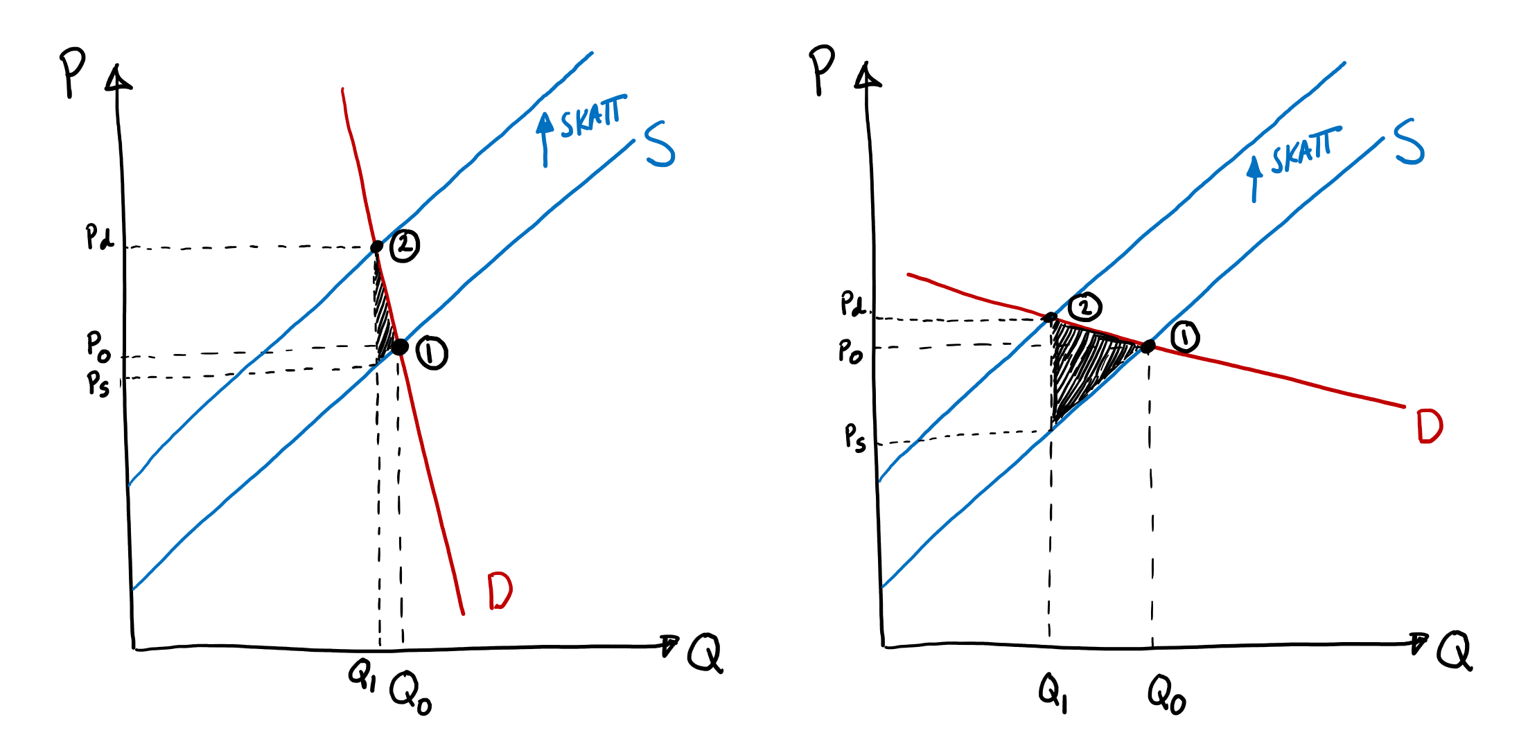
In both panels above I’ve drawn identical supply curves and in both cases we start from equilibrium 1, where the price is P0 and the quantity is Q0. Note, however, that the demand curve is steeper in the left panel than in the right, which indicates that those consumers are less price‑sensitive.
Now I introduce a tax into the analysis, which can be illustrated by shifting the supply curve upward by the amount of the tax. Do you see what happens? In the left panel, where consumers are less price‑sensitive (think “more desperate”), a larger share of the tax will in practice be borne by consumers. In the right panel it is instead the firms that end up bearing the larger part of the tax burden.
Who legally remits the tax to the authorities is therefore completely irrelevant. In the political debate there are currently calls for a special bank tax — but few probably realise that much of that tax will ultimately be shifted onto everyone who has a bank account. In practice the tax burden is always distributed so that the least price‑sensitive party bears the largest share. The desperate are often exploited in life, and the same holds in tax analysis: if customers are desperate it is easier for firms to pass a larger part of the tax on to them (since they keep buying even when the price rises).
tax incidence concerns who actually bears the tax burden (regardless of who legally remits it)
Note also that tax revenue is larger and deadweight loss smaller in the left panel than in the right. Why? Because consumers there are insensitive to price increases. They continue to buy even when the state imposes a tax. In the right panel a large share of trade is destroyed by the tax, so there is less trade left to tax. From a pure efficiency perspective it is therefore better to tax goods and services with inelastic demand — housing, life‑saving cancer medicines, etc. On the other hand, society may be willing to sacrifice some efficiency for goals we consider more just.
Tax on labour: Do higher tax rates raise more revenue?
I have noticed many times that economists think differently than others. Here are three examples:
100 litres of strawberries are sold at the Market Square every day. Municipal politicians now want to introduce a tax that forces firms to pay €1 for every litre they sell. The politicians think this will raise €100 in tax revenue. The economist expects it will be less than €100.
A firm is considering making occupational health services free for employees. But what would such a reform cost? Last year employees used the occupational health service a total of 1,000 times, and each visit cost €100. Management therefore says the reform would cost the firm €100,000. The economist thinks it will cost more than €100,000.
A university course has 100 students. The probability of passing the exam is 90%. To increase throughput the university now introduces an additional exam session, which costs taxpayers about €1,000 in extra administrative and labour costs. Management defends the reform and claims that the extra session will bring the pass rate to 99 out of 100 — that is, 90 students pass at the first sitting and an additional 9 at the second. The economist thinks fewer than 99 students will pass.
What makes the economist reach completely different conclusions than the other politicians and social scientists? I think it stems from viewing how choices respond to changed incentives. The tax will scare some customers away from the market, so tax revenue will be smaller. Free occupational health care will make more people visit the doctor, so health‑care costs will rise. The possibility to resit an exam will lead fewer students to turn up at the original sitting.
You can use the same logic to think about how higher taxes on labour affect government revenue. Higher taxes will — according to our analysis — make fewer people want to work. Theoretically, therefore, lowering labour tax rates could increase tax revenue. The relationship between the tax rate and tax revenue is called the Laffer curve. Economist Arthur Laffer sketched the relationship on a napkin when discussing tax policy with influential US politicians in Washington in the 1970s. He drew his curve roughly like this:
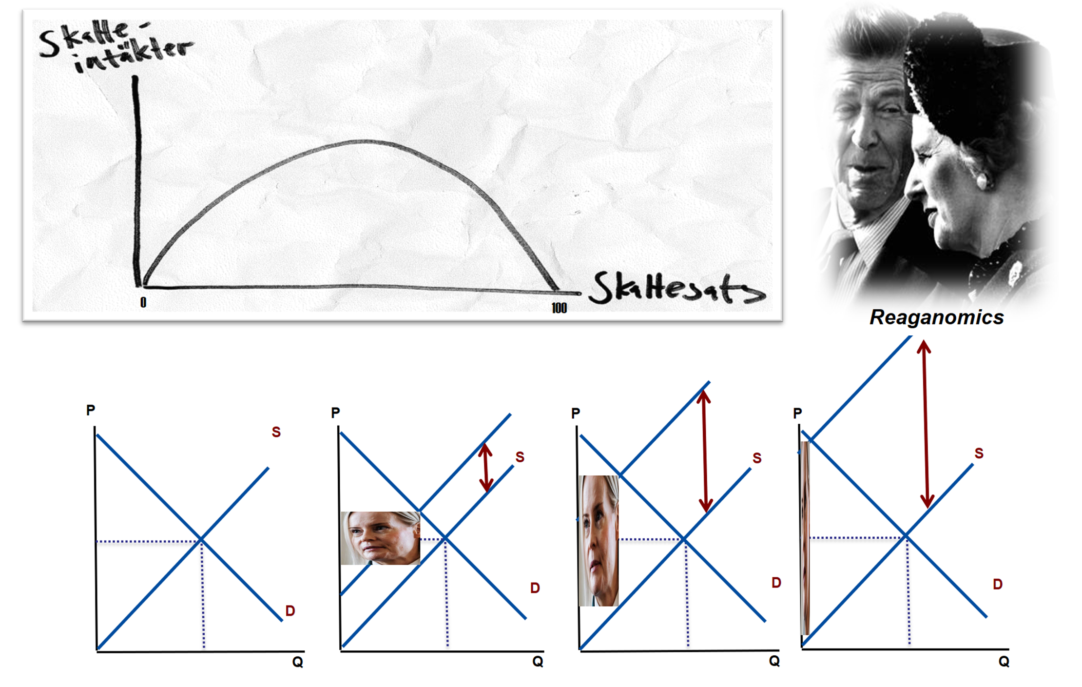
When the tax rate is 0 the government naturally collects no tax revenue, but the same is likely true when the tax rate is 100% because hardly anyone would work if the state took all wages. That implies there must be some tax rate between 0 and 100% at which revenue is maximised.
If we are “to the left” of that rate, tax revenues rise when rates increase; but if we are “to the right” of that point, then a cut in tax rates can increase tax revenue. An interesting research question is therefore to determine whether a given country lies to the left or to the right of the revenue‑maximising point.
The Laffer curve had a huge impact on economic policy worldwide and helped drive many labour‑tax cuts in recent decades. The curve was central to President Reagan’s economic policy in the 1980s. In an exercise at the end of the chapter Laffer himself explains more about his famous curve. It’s a remarkable display of political lobbying.
Subsidies are a reverse tax
Taxes reduce trade. A tax on e‑bikes therefore makes fewer e‑bikes sold. But suppose, as finance minister or a municipal politician, you want more people in Turku to buy e‑bikes — for public health or to reduce car traffic around the Market Square. How do you achieve that? The answer is a subsidy. Think of a subsidy as a reverse (negative) tax: instead of firms paying a fee per unit they sell, they receive money for each unit sold. Because a tax shifts the supply curve left, a subsidy shifts the supply curve right. The effect is the mirror image of a tax: trade increases (and becomes inefficiently large), the consumer price falls, firms receive more (after accounting for the subsidy), and the government incurs a large expenditure to subsidise all the transactions.
Exercises
In this chapter you learned how politicians can intervene in markets using economic‑policy tools to change prices or the quantities produced and consumed. Below you can practise this type of exercise. As usual, press Show Answers when you want the computer to grade your responses. Good luck!
Taxes kill
You will now analyse how a tax affects the market for loaves of bread. An important lesson is that taxes kill. The following figures show how the market looked before taxes were introduced. You can see that the market price is €2 per loaf and that 100 loaves are sold.
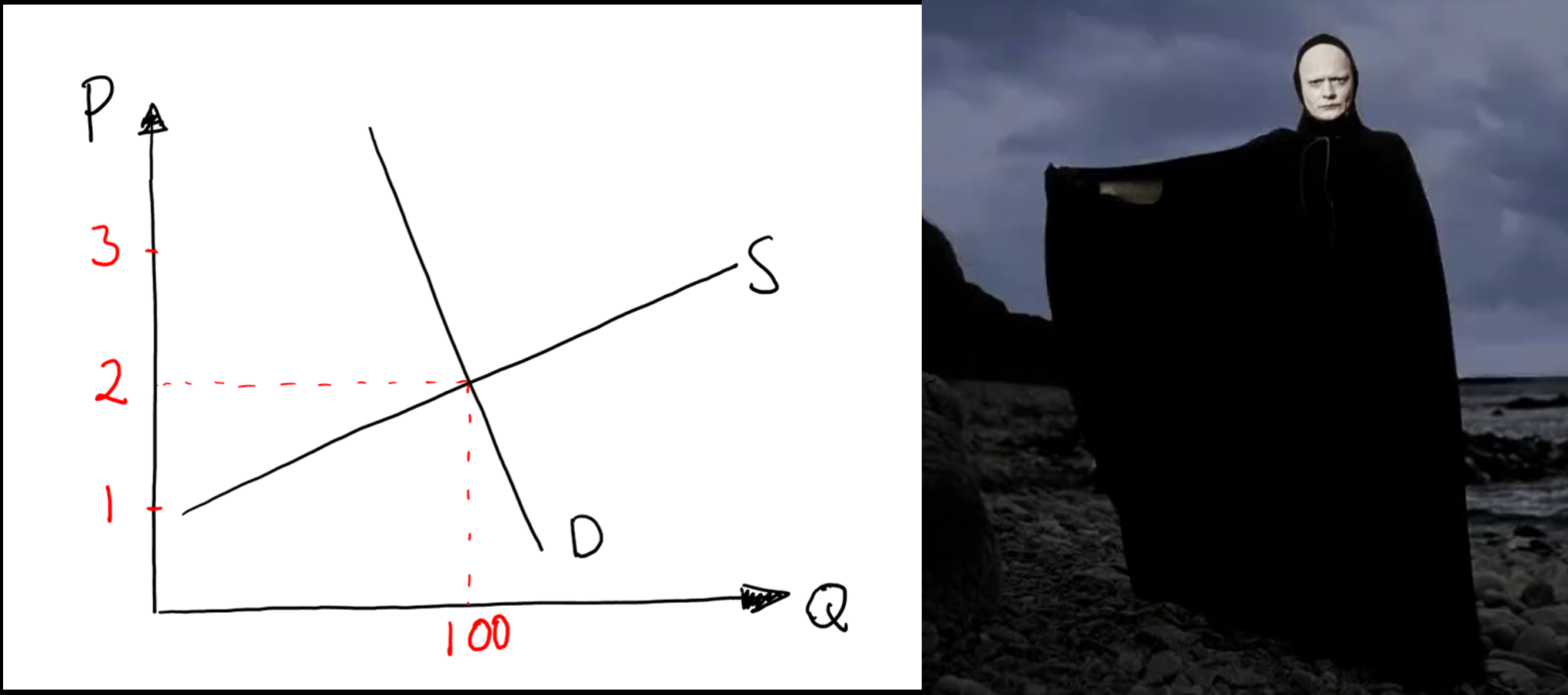
- Imagine the government now imposes a tax of €1 per loaf. Producers are legally required to remit the tax to the government. What happens in the figure above when the state hits firms with this levy? Answer: .
- The price in the shop paid by the customer .
- The price received by sellers after the tax .
- The group that in practice bears the largest share of the tax is , which is because that group is the most desperate and therefore much of the tax can be “shifted” onto them.
- Imposing a €1 tax in a market where 100 loaves were originally sold therefore yields tax revenue that is .
- Now assume administratively the tax is levied on consumers instead of producers — i.e. consumers remit the €1 to the government each time they buy a loaf. What happens in the figure above then? Answer: .
- The price the seller receives .
- The price the buyer pays once she has also remitted the tax .
- Anything that makes life worse for firms will reduce supply: at each price level firms will want to offer less than before.
- Of a €1 tax, €0.80 ends up on the customer. Consumers therefore bear 80% of the tax burden.
- Of a €1 tax, €0.20 ends up on the customer. Producers therefore bear 20% of the tax burden.
- Think for a few seconds about what this implies. For example, consider the firm you started in the exercise in Chapter 3. Do you think customers in that industry have an inelastic demand? That can happen if your product is unique or perceived as unique (think: “consumers are brainwashed by advertising”). In that case you can pass a large share of the tax onto customers because most will continue to buy the product even when it becomes more expensive.
- Remember that taxes kill trade — which shrinks the tax base; there is simply less trade left to collect tax revenue from.
- So far we assumed firms legally remit the tax, but in this exercise consumers remit the tax to the government. Something must therefore happen to the demand curve. Recall that the demand curve shows the price that makes consumers want a given quantity. For example, for consumers to want 100 loaves the price must be €2 per loaf. What if consumers must also pay a €1 fee per loaf? Then the store price that makes consumers still want 100 loaves must fall to €1. Buying a loaf for €2 (tax‑free) is the same as buying it for €1 and then remitting €1 to the authorities. So shift the demand curve down by the tax amount.
- Read off the new equilibrium. That is the shop price — the price sellers receive before any tax remittance.
- The shop price is not the buyer’s final price, because the buyer still must remit €1 to the state. Move up to the original demand curve (which lies €1 higher) to read the buyer’s final price (after tax). One lesson is that it is practically irrelevant, in economic incidence terms, whether the tax is administratively levied on producers or consumers.
Interventions in the market for used coursebooks
At the end of Chapter 3 you launched a marketplace for trading used coursebooks. Your platform has been a big success. Demand is given by \(\small Q_D=7,000 - 100P\) and supply by \(\small Q_S=50P - 500\), where Q is the number of books and P is the price in euros. For simplicity we assume all books sell at the same price.
- In equilibrium the price is per book and the quantity traded is .
However, increasing calls are being made for various interventions in the market. You will now analyse how each intervention would affect the market:
- The Student Union has complained loudly. They think the market price is unreasonably high. “All students must be able to afford coursebooks,” they claim. They therefore demand that the authorities impose a price ceiling of €30 per book. If the price ceiling is introduced, books will be sold; producer surplus (PS) falls from euros to euros, and consumer surplus (CS) increases from euros to at most euros.
- The Association for Active Youth also complains. They believe young people should be outdoors rather than reading textbooks. They therefore demand that the authorities impose a quota of 1,000 books. Suppose the quota is introduced. The market price would then be , which results in a deadweight loss of euros.
- You yourself want to introduce a fee on the market (think “tax”): each time a book is traded the seller must pay you €6. The effect of such a fee is that trade falls to , the price for buyers rises to , sellers receive per book after the fee, and your total revenue from the fee is euros.
- Set \(\small Q_D=Q_S\) and solve for the price that makes consumers want to buy exactly as much as producers want to sell.
- This is a tricky problem. Draw the diagram and take it step by step. At P = €30 the supply curve indicates sellers want to supply 1,000 books, so that will be the traded quantity (you cannot force sellers to sell if they won’t). In the initial equilibrium PS was the large lower triangle with area €40,000 (base 2,000 × height 40 ÷ 2). When the price ceiling €30 is imposed PS falls to €10,000 (new triangle base 1,000 × height 20 ÷ 2). Initial CS was €20,000 (base 2,000 × height 20 ÷ 2). To compute the new CS note it equals a large rectangle plus a small triangle: find the price at which consumers would buy 1,000 books by plugging Q = 1,000 into inverse demand, \(\small P_D=70 - 0,01*1\,000=60\). The small top triangle area is €5,000 and the large rectangle area is €30,000, so CS = €35,000.
- The new market price (after the quota) is €60. To compute the deadweight loss first find the seller price at Q = 1,000 by plugging into inverse supply: \(\small P_S=10 + 0,02*1\,000=30\). You now have the numbers to compute DWL: it is the area of the triangle with base 1,000 and height €30 (use the triangle area formula).
- As always, draw the figure yourself. Think of yourself as the platform owner (the “state” in this exercise). Imposing a €6 fee on sellers shifts the supply curve up by €6. Solve \(\small 10+0,02Q+6 = 70-0,01Q\) to get Q = 1,800. The buyer price at Q = 1,800 is \(\small P_D=70 - 0,01*1\,800=52\). Sellers’ net price after remitting the fee is €46. Your fee revenue equals 1,800 × €6 = €10,800.
Rent control in the housing market
It is easy to get a first‑hand tenancy in central Turku, but almost impossible in Stockholm city. Why is that? Suppose the sketch below shows supply and demand for small rental apartments in Turku. If you want to read more about the housing markets in Sweden vs Finland you can read here.
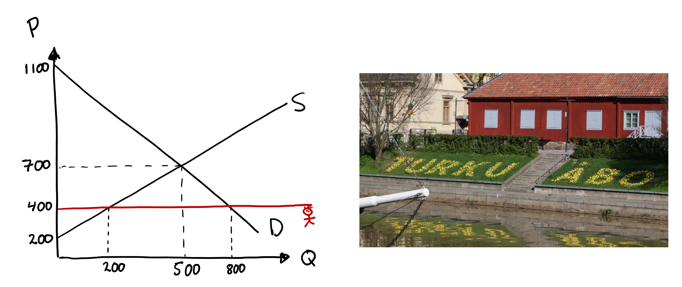
- Explain in your own words why the rent for the flat in Turku will be €700, given that we have not introduced a price ceiling.
- Without a price ceiling the consumer surplus (CS) in the figure is . In your own words, explain what that number means in plain language.
- Without a price ceiling the producer surplus (PS) in the figure is . In your own words, explain what that number means in plain language.
- Student organisations are furious: it is unreasonable that small flats should cost €700 per month — students can’t afford that! They therefore demand a price ceiling of €400. If the ceiling is introduced the number of flats actually rented will be , while the number of flats demanded at that low price will be .
- In your view, how should the authorities allocate the 200 flats among the 800 people who want them?
- Think about what would happen if the price were not €700 but, say, €400 or €900.
- Explaining CS is not easy. Write your answer on paper so you’re not doing it for the first time under exam stress. A full‑credit answer could be: “The consumers who bought on the market collectively valued their purchases €100,000 more than the price they actually paid.” Include the word “euros.” Be precise and clear.
- Practice phrasing a good answer. Write it down and read it back: is it clear and exact? Include “euros.” Example: “The sellers who sold on the market collectively received €125,000 more than the minimum they would have accepted.”
- What would happen in an unregulated market if the price were €400? (Hint: demand would exceed supply, so shortages and non‑price allocation would appear.)
- How should the authorities allocate 200 flats among 800 applicants? Options include: lottery, queues, prioritized need-based allocation, application scoring, or corrupt methods. Think about fairness, efficiency and political feasibility when you choose.
Minimum wage
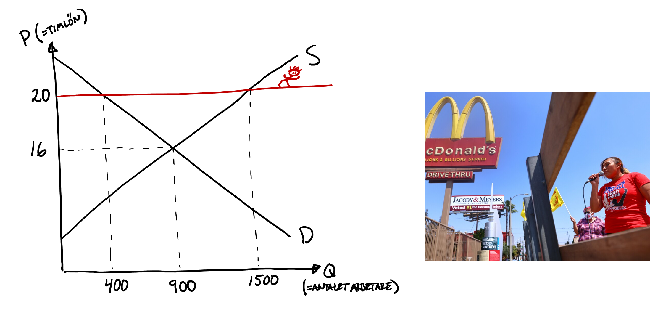
On 1 April 2024 California suddenly raised the minimum wage for all fast‑food workers from $16 to $20. In this exercise you will show what effects this reform is likely to have. First watch the short news clip about the reform:
- The figure below is a sketch of the labour market in a Californian city. Does the law of supply hold, given that no minimum wage has been introduced? Answer: .
- Why is the wage $16 per hour when we do not have a minimum wage? Explain!
- The union protests: “It is unreasonable that workers should earn only \(16\) per hour. Workers, often students, cannot afford to live!” The union therefore demands a $20 minimum wage. If the minimum wage is introduced, the number of workers restaurants hire will be , while the number of people willing to supply their labour at this higher wage will be .
- How should the 400 jobs be allocated among the 1,500 people who want them, in your view?
- Are you for or against higher minimum wages? Answer: .
- Do more people want to work when the wage rises?
- What would happen if the hourly wage were not $16?
- Note that minimum wages thus cause unemployment.
- Interviews? Time spent unemployed? Lottery? Personal contacts?
- This depends on your values — there is no single right or wrong answer.
Finland raises VAT on 1 September 2024
On 1 September 2024 Finland raised its consumption taxes. Previously VAT was typically 24 percent; it was suddenly increased to 25.5 percent. In this exercise you will consider how the higher taxes affect prices in shops.
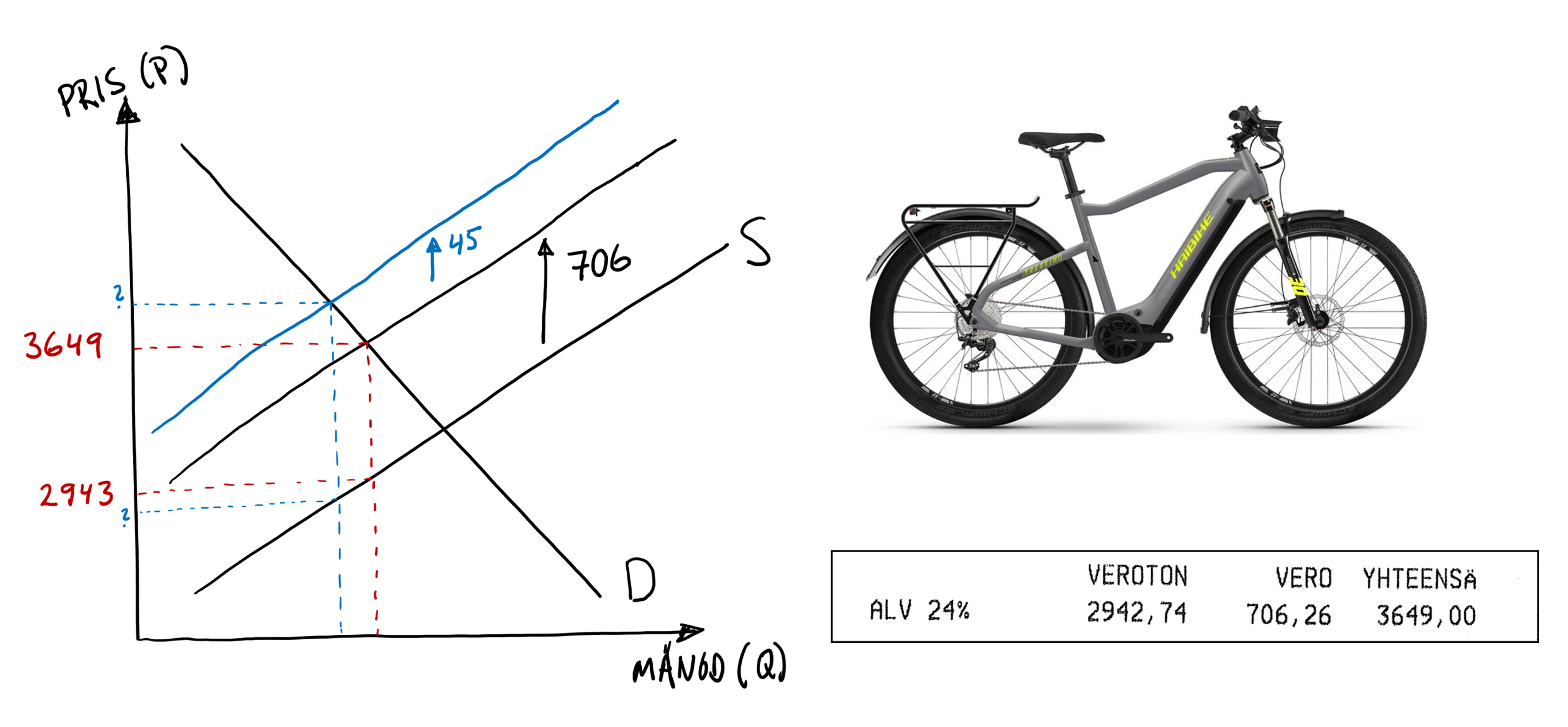
- What does theory predict will happen to shop prices when VAT is raised? Explain in simple terms.
- Before the reform, when VAT was still 24%, I bought an e‑bike. In the figure I illustrated the equilibrium in red: the tax (about €706 on my bike) made the consumer price €3,649 while the shop kept €2,943 after remitting the tax. The VAT increase meant the tax rose by roughly another €45. What will likely happen to the shop price when VAT is raised? Answer: .
- How will the VAT increase likely affect how many e‑bikes are sold? Answer: .
- Explain in your own words: what determines how large a share of the €45 tax increase shops can pass on to customers?
- Explain in your own words: do you think the e‑bike shop can pass a larger share of the VAT increase onto consumers than the flower shop Tähkä can? Motivate your answer.
- The tax will probably raise the shop price but not by the full amount of the tax. The burden is shared between customers and firms. Exactly how it is divided depends on price elasticities: the side that is least price‑sensitive bears the larger share of the tax.
- See hint 1.
- See hint 1.
- Write down a clear answer on paper. In the exam you won’t have time to think it through — it must come to you immediately.
- Write down a clear answer on paper. In the exam you won’t have time to think it through — it must come to you immediately.
Subsidy for higher education
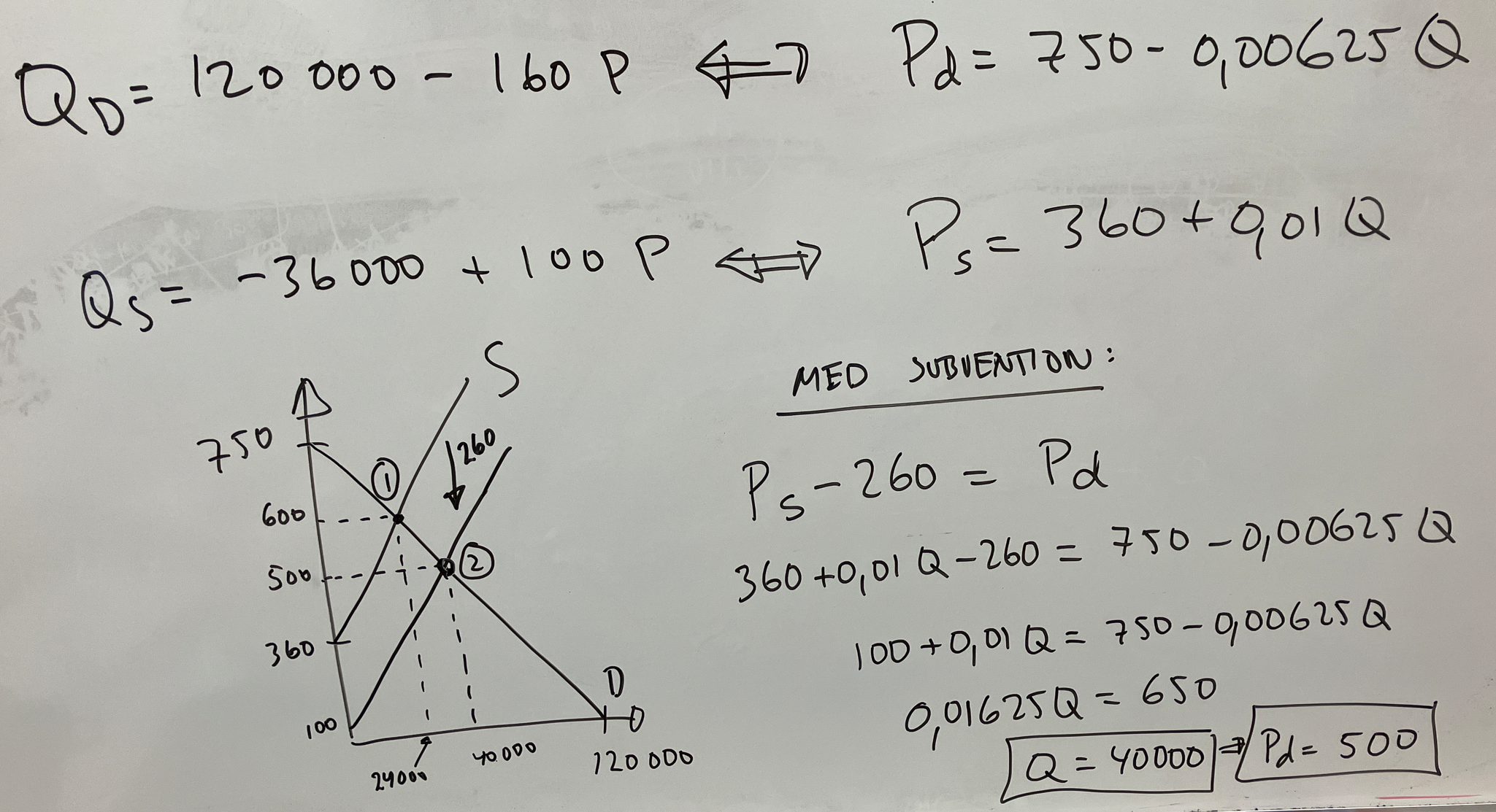
In a country all university education is provided privately. Demand and supply are given by \(\small Q_D=120{,}000-160P\) and \(\small Q_S=-36{,}000+100P\), respectively, where Q is the number of study places and P is the tuition fee per term in dollars.

- The market tuition fee will be and the number of students will be .
- To get more students to study, the government now subsidises each place by $260. The new tuition fee paid by a student therefore becomes .
- Many other groups in society also need financial support. What is the total cost to the state of subsidising education? Answer: .
- See the solution below. Set Qd = Qs and find the price that ensures universities want to sell as many study places as students want to buy. Illustrate the solution to make it easier. Taking the inverse functions is useful for the future. \(\small Q_D=120,000-160P\) can be rewritten as \(\small P_D=750-0,00625Q\) and \(\small Q_S=-36,000+100P\) as \(\small P_S=360+0,01Q\).
- Imagine that universities receive $260 for each student. This will shift the supply curve down by the size of the subsidy (a tax shifts the supply curve up and a subsidy is the opposite of a tax). The new supply curve therefore becomes \(\small P_S=100+0,01Q\). Now you can calculate the new tuition fee for students.
- You can calculate that the number of students increases to 40,000 thanks to the subsidy. For each student the universities should receive $260.
The Tax on Labor
Economists often have a very large influence on policy. In this video clip the economist Arthur Laffer discusses how it happened when he first drew the Laffer curve on a napkin, thereby influencing tax policy in the United States and in large parts of the world.
- What does the Laffer curve say? Summarize in one sentence!
- Do you think that higher taxes on labor in Finland would make tax revenues increase or decrease?
- Write down a good answer. Note that Laffer draws his curve with the tax rate on the vertical axis and tax revenue on the horizontal axis, but that is a matter of taste.
- This is an interesting research question. In, for example, the course Arbetsmarknadsekonomi you will learn much more about different phenomena in the labour market.