15 Fiscal policy
(where you learn how politicians can steer the economy by accelerating and braking)
In the previous chapter you got an introduction to business‑cycle analysis. One important insight was that GDP in the short run depends on aggregate demand. If households and firms, for some reason, no longer want to consume and invest as much as before, GDP will fall in the short run. In the long run the economy, however, self‑heals: prices and wages adjust so the economy recovers and we are automatically pulled back to the long‑run GDP level.
Here is an analogy that may help you understand the mechanism. Imagine three saucepans of boiling water. Each saucepan has two outlets: P and Y. When the water boils steam is produced and must escape. But where does it go?
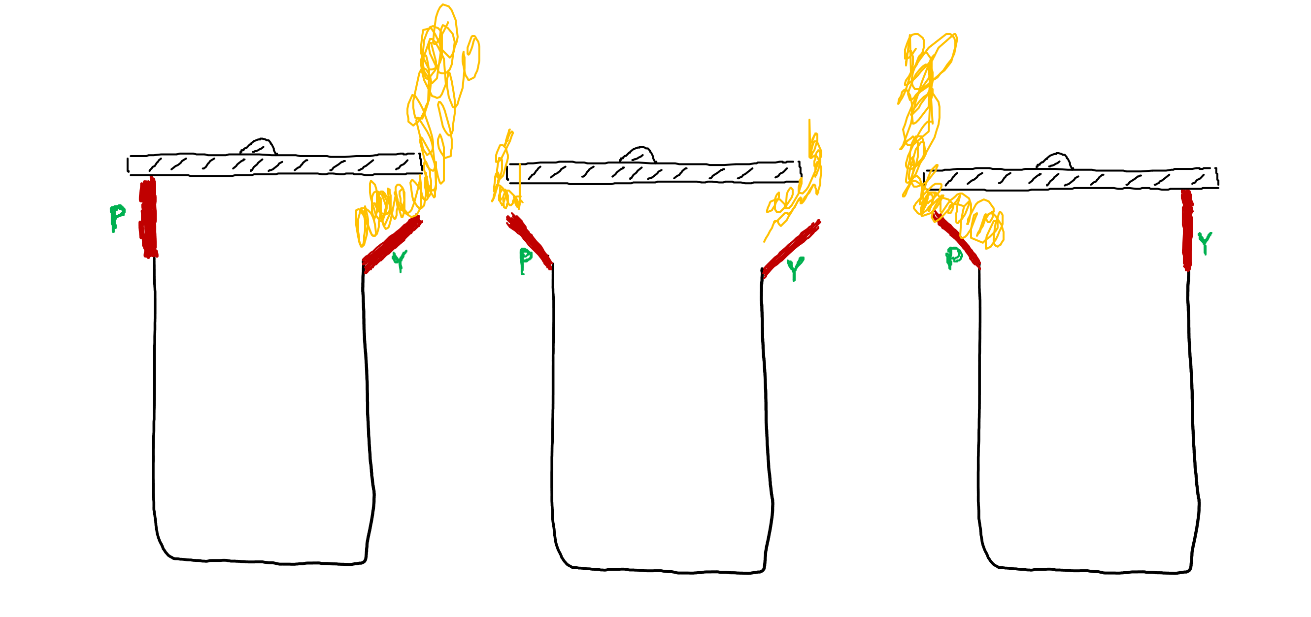
In the saucepan on the far left we have closed the P outlet. All the steam therefore shoots violently out through the Y outlet — there is simply nowhere else for it to go because P is “locked”. In the saucepan on the far right the Y hole is closed, and all the steam flows out through the P outlet. In the middle saucepan both holes are open, so a little steam comes out of both P and Y. Do you see the analogy between the saucepans and Figure 14.5? The boiling water is the energy released when five million Finns suddenly feel more optimistic about the future. It is the force of 250 coffee‑hungry students storming Fabbe’s café.
In the very short run prices are locked — and production must take the full impact. In the short run Fabbe has more room to manoeuvre and he uses the opportunity to raise his prices. When he charges more some students are deterred, which dampens the frenzy a little, but the café is still booming. In the long run it is Y that is effectively locked: you simply cannot produce more than is sustainable over the long term. Hence in the long run only the price level is affected by the demand shock.
15.1 What is fiscal policy?
It is 14 September 2001 and President Bush visits Ground Zero in New York. He urges Americans to carry on as usual after the terrorist attacks. Why does he say this? Perhaps he fears that panic in the US will trigger a sharp fall in consumption and investment — and thus a devastating recession?

Could the president have done more?
Let’s return to the circular flow. You know from the previous chapter that a country’s output in the very short run is determined entirely by how much we want firms to produce (Y = AD) — but how can President Bush influence aggregate demand? Imagine Bush sitting in the middle of the circular flow with the power to steer the government’s spending and revenues.
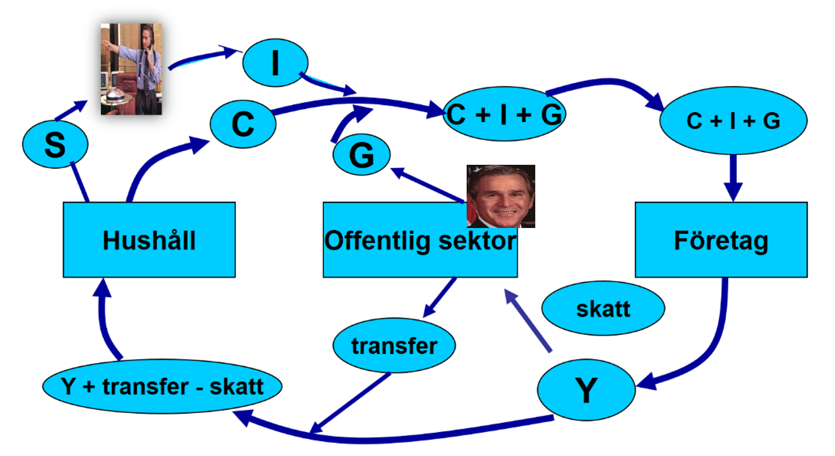
One direct measure would be to increase government consumption (G). For example, he could ensure the state expands defence spending or makes large investments in schools and healthcare.
But Bush can also influence how much households want to consume. If he cuts taxes and/or raises transfers, households’ disposable income rises and, with more money in their pockets, they will likely spend more.
All this — changing government consumption (G), taxes (T) and transfers (Tr) — is called fiscal policy. The aim of fiscal policy is often to stabilise the economy around its long‑run trend. Most of us prefer to live in a country that isn’t violently tossed between good and bad times. Fiscal policy is an important tool George can use to pursue this stabilisation policy.
fiscal policy is about how the government uses its spending and taxes to influence the economy; by adjusting taxes, transfers and public consumption policymakers try to stabilise the economy around the long‑run GDP level (the same goal can also be pursued via monetary policy in Chapter 18).
Government spending
The figure below shows how public spending (as a share of GDP) has evolved in Finland over history. As always, you can click Map to view the whole world, or add individual countries via Edit countries and regions.
As you can see, public spending has risen sharply over time and now exceeds half of our GDP. The share increased markedly during the wars and the 1990s crisis. The public sector — that is, central and local government — has therefore come to play an ever larger role in our lives.
What do these public expenditures consist of? Below you can see the figures for Finland in 2024. The largest item is “social protection”, which includes payments to the sick, the elderly and the unemployed. Other major spending categories are healthcare and education. Infrastructure is also important; it is by no means free to build railways, motorways or a town‑centre car park.
| SpendingArea | Per capita, euro |
|---|---|
| Allmän offentlig förvaltning | 3513 |
| Försvar | 761 |
| Samhällskydd och rättsskipning | 648 |
| Näringslivfrågor | 2397 |
| Miljöskydd | 107 |
| Bostadsförsörjning och samhällsutveckling | 258 |
| Hälso- och sjukvård | 3795 |
| Fritidsverksamenhet, kultur och religion | 815 |
| Utbildning | 3072 |
| Social trygghet | 12988 |
Some of these expenditures are negotiated in the annual budget. Should the money go to a town‑centre car park or to care for the elderly? Should study grants be raised or should funds be used to reduce class sizes?
But politicians cannot change large parts of spending. Many expenditure items are set in law. For example, all children have the right to attend school and all elderly people have the right to a pension. These laws are very hard to change. That is one reason so many are worried about the development of Finland’s demographic dependency ratio.
a budget is a plan for next year’s revenues and expenditures
transfers are monetary payments from the state and municipalities to households, firms and organisations
Government revenues
How can the public sector finance all its spending? By collecting taxes. How the tax system works is a huge topic we touched on in Chapter 5, but a few terms are useful to know. Imagine the tax system looks like this:
| Income (euros) | Marginal tax (%) |
|---|---|
| Under 100 | 10 |
| 100 - 200 | 50 |
| Over 200 | 102 |
This means that all income up to €100 is taxed at 10 per cent. You then pay 50 per cent tax on any income between €100 and €200. Everything above €200 is taxed at 102 per cent. So how much tax do you pay? Well, that depends on how much you earn.
| Individual | Income | Marginal tax (%) | Tax (euros) | Tax (% of income) |
|---|---|---|---|---|
| Adam | 90 | 10 | 9 | 10 |
| Eva | 150 | 50 | 35 | 23 |
| Astrid | 250 | 102 | 111 | 44 |
Look first at Adam, who earns €90. Since everything under €100 is taxed at 10 per cent, Adam pays €9 in tax — which is 10 per cent of his income. For Eva, who earns €150, it’s a bit trickier. On her first €100 she pays 10 per cent (= €10), but once she crosses the €100 threshold the tax rate on the next euros rises — the marginal tax rate becomes 50 per cent. For the €50 she earns above €100 she therefore pays half in tax (= €25). In total Eva pays €35 in tax, which is about 23 per cent of her income. At the bottom of the table is Astrid, an 80‑year‑old children’s author from Sweden who has just written the bestseller The Brothers Lionheart. Astrid has therefore earned huge income. Can you check that about 44 per cent of her income goes to tax?
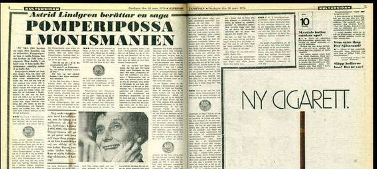
This very example is said to have decided the Swedish parliamentary election in 1976. Astrid Lindgren was — on the margin — taxed at more than 100 per cent. Many therefore argued that Astrid lost money by working.
Can you argue against that claim by referring to the concept of the marginal tax rate?
Look back at what Adam, Eva and Astrid pay. You see that those who earn more also pay a larger share of their income in tax. This is therefore an example of a progressive tax system. The opposite is called a regressive tax system, and a system where everyone pays the same share of their income in tax is called a proportional system.
Taxes are not only levied on income but also on consumption. Every time you fill your car you pay tax. The petrol might actually cost €0.50 per litre; the rest is tax. In the same way you pay tax whenever you buy other goods and services.
There is a perpetual debate about how the public sector should finance all its spending. Many argue that income taxes reduce labour supply and that high marginal tax rates deter people from, say, writing children’s books. Others argue that income taxes are fairer than consumption taxes. Take milk as an example. Most of us buy roughly the same amount of milk (the billionaire does not buy 1,000 times more milk than you). If the public sector relied solely on a milk tax, the poor student would pay about the same number of tax euros as the billionaire — which would make the system regressive.
15.2 Fiscal policy: the intuition
The intuition behind fiscal policy is simple: the public sector can influence the business cycle by accelerating or braking the economy. Two central concepts are worth remembering: 1) Lean into the wind and 2) the multiplier effect.

Lean into the wind means George must spend big when nobody else dares and restrain spending when everyone else is splashing out. It’s like Bush at Ground Zero thinking: people are cutting consumption and firms won’t invest — the state must uphold demand to avoid a deep recession! So the government buys motorways, fighter jets, expands schools and care homes. George also cuts taxes and raises transfers — with more money in people’s pockets they are likelier to buy a new car or eat out. All this supports AD and may prevent the US from plunging into a recession with high unemployment and low incomes.
The problem is these measures cost the public purse. George voluntarily reduces tax revenues while increasing transfers and public spending. The result is a budget deficit — and to finance it the government must borrow.
If the country then moves into a boom — with spendthrift consumers and over‑optimistic firms — George should instead prevent overheating by raising taxes and cutting public spending. That will probably produce a budget surplus, which can be used to pay down the debts accumulated during the downturn. This is roughly how Keynes thought fiscal policy should operate to help people like Tom Joad.
The second key concept is the multiplier effect. Suppose George wants to raise GDP by EUR 100 million. He decides to build a town‑centre car park costing EUR 100 million. What happens?
In the very short run AD determines GDP. If George demands a car park, he gets a car park. But that’s only the start. A EUR 100 million rise in GDP means incomes rise by EUR 100 million. Let’s ignore taxes and transfers and assume households spend half of any income increase. When households receive EUR 100 million they will spend EUR 50 million on goods and services. Firms respond: in round 2 GDP increases by another EUR 50 million. George’s initial EUR 100 million order thus produced EUR 100 million of construction plus EUR 50 million of other goods and services. It doesn’t stop there: in round 3 households’ incomes rise by EUR 50 million, they spend EUR 25 million, firms respond, and so on.
Round after round the economy spins: 100 + 50 + 25 + 12.5 + 6.25 + 3.125 …
This is the multiplier effect: the final impact on GDP is larger than George’s initial change in AD. So if George wants to raise GDP by EUR 100 million he does not need to increase public spending by the full EUR 100 million — his initial stimulus triggers a snowball effect that he must account for when designing stabilisation policy.
But idiots who shower and politicians who cheat
Imagine you step into the shower and turn on the tap. It may take a few seconds for the water to arrive, especially if the pipes are old. You scream in panic. The water is scalding hot! You yank the tap fully the other way to make it colder. Cold water rushes through the pipes and a few seconds later: another scream! The water is freezing! You lunge for the tap again and twist it fully in the opposite direction. This is the story of the idiot in the shower.
Why does this happen and what does the idiot in the shower have to do with Finland’s fiscal policy? The problem is that water temperature doesn’t change immediately when the idiot turns the tap — and George faces the same time‑delay problem. He wanted to raise GDP to rescue the country from recession and therefore pulled the lever for expansionary fiscal policy. But building a town‑centre car park does not happen in an afternoon. First you must apply for permits and hire architects. Then construction firms must bid. Environmentalists appeal; there are demonstrations and court cases. Three years later you put a spade in the ground, but the project must be paused when unique Viking‑era finds are discovered. Moreover, the multiplier effect means it takes time for the full impact to appear in the economy.
The danger is that the economy will have already self‑healed by the time the expansionary policy finally kicks in. George meant to save the economy from recession — but all he achieved was to stoke the boom. The time lag is as devastating for George as for the idiot in the shower.
Another analogy that may help you remember the difficulties of fiscal policy is steering a Viking Line ferry. It takes a long time to get the colossal ferry to turn. If you want the ferry to be 200 metres to the right ahead, you must start turning the wheel now — otherwise you will be too late. To avoid running aground you must know what lies ahead and act early. The same applies when steering Finland’s economy.
In fiscal policy people often talk about the three Ts: timely, temporary and targeted. The difficulty is to implement measures at the right time (timely). Ideally the measures should also be temporary (temporary). For example, politicians might raise study grants during a pandemic to support demand — but can they really bring study grants back down to the original level when the pandemic is over? Measures should also be well targeted (targeted): if the aim is to stimulate consumption it is probably much more effective to give €100 to a family with children than to a billionaire. The family will likely spend a large share of the €100, whereas the billionaire will simply deposit it.
In theory it is possible to use fiscal policy so the economy always sits at potential output, but the three Ts show it is extremely difficult: George must know exactly where the economy is headed and then apply exactly the right dose at exactly the right time. Fine‑tuning the economy week by week easily goes wrong: one week you build car parks to boost demand, the next week you cut study grants to cool the economy. Most economists therefore argue this kind of fiscal fine‑tuning should be reserved for truly large crises or when the economy is extremely overheated.
But what if you could find a clever way so George does not have to pull any levers? What if the public sector automatically distributed more money in crises and collected more in good times? If you think about it you may realise this is exactly how tax and benefit systems are normally designed. In bad times with lower incomes you pay less tax (think back to Adam, Eva and Astrid) and if you become unemployed you receive unemployment benefits. In good times the progressive tax system means the state automatically takes a larger share of your income — and fewer people qualify for benefits.
This kind of countercyclical fiscal policy is called automatic stabilisers. Compare these with discretionary fiscal policy, where George himself must pull the levers for anything to happen. When do you think the time‑lag problem is worst?
Another concern is fiscal policy abuse. Public Choice is an interesting research field that analyses politics using economists’ tools. Imagine the following scenario: you are a politician in a small Finnish municipality. The last election went well and you’ve governed for three years. A new election is approaching. From your economics studies you remember that expansionary fiscal policy raises incomes and lowers unemployment in the short run. You also recall Bill Clinton’s phrase that pocketbook issues often decide how people vote — “It’s the economy, stupid!” — and that many historians argue the German electorate brought Hitler to power in 1933 largely because the economy was in chaos.
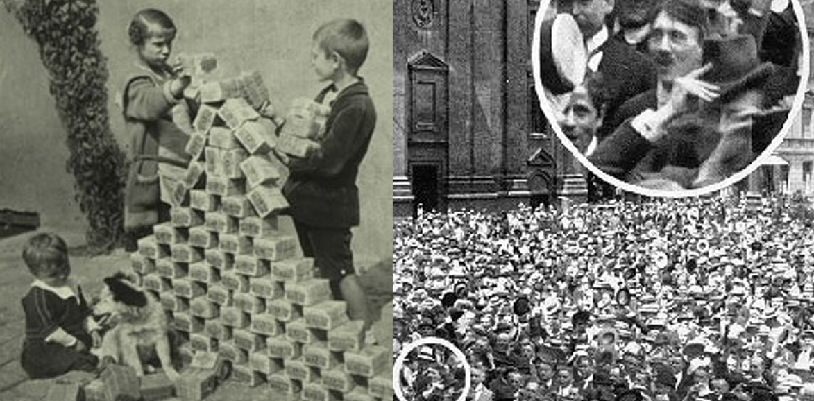
Hand on heart: is there a risk that you as a politician don’t do what is best for the municipality in the long run — but instead selfishly pursue expansionary fiscal policy to maximise your own chances of re‑election?
If politicians act this way the economy will often boom precisely on election day. We then get so‑called political business cycles. Is there evidence that politicians actually abuse their power for personal gain? In the table below Dahlberg & Mörk (2008) followed all municipalities in Finland and Sweden for about 18 years and examined whether anything special happens to fiscal policy around election years. The results are clear: in election years municipalities on average hire more people, increase public consumption and cut taxes.
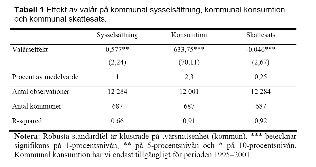
This pattern may of course have explanations other than politicians abusing power, but isn’t it a strange coincidence that it is so often during election years that politicians pull the lever for expansionary fiscal policy?
These signs of misuse of power have prompted some to argue that control over fiscal policy should be limited or even removed from politicians. For example, rules requiring the budget to be balanced over a multi‑year horizon have become more common.
Do you think it is economically wise to legislate budget balance? It may curb some abuse of power but also forces politicians to cut sharply in crises — which likely deepens those crises. And is it democratically acceptable to strip elected officials of economic tools?
15.3 Fiscal policy: the math
We have now covered fiscal policy on an intuitive level. Hopefully you understand the core ideas. We can now take another step and do some calculations. The app below is a slightly more advanced version of the app you used in the previous chapter. Do you see the difference? Here I have also included taxes and transfers in the model. Play with the app for a while until you understand how it works. Note that you must always press the “Calculate and illustrate” button for the app to compute the new equilibrium.
#| standalone: true
#| viewerHeight: 1360

if (!requireNamespace("shiny", quietly = TRUE)) install.packages("shiny")
if (!requireNamespace("plotly", quietly = TRUE)) install.packages("plotly")
if (!requireNamespace("grid", quietly = TRUE)) install.packages("grid")
if (!requireNamespace("scales", quietly = TRUE)) install.packages("scales")

library(shiny)
library(plotly)
library(grid)
library(scales)

safe_numeric <- function(x, default = 0) {
  if (is.null(x) || identical(x, "") || is.na(as.numeric(x))) return(default)
  as.numeric(x)
}

# Helper for consistent formatting
fmt <- function(x) comma(x, accuracy = 0.01, decimal.mark = ".", big.mark = ",")

ui <- fluidPage(
  fluidRow(
    column(4,
      wellPanel(
        numericInput("a", "Autonomous consumption (a):", value = 100, min = 0, step = 1),
        numericInput("b", "Marginal propensity to consume (b):", value = 0.8, min = 0, max = 0.99, step = 0.01),
        numericInput("I", "Investment (I):", value = 50, min = 0, step = 1),
        numericInput("G", "Government spending (G):", value = 80, min = 0, step = 1),
        numericInput("c", "Autonomous tax (c):", value = 10, min = 0, step = 1),
        numericInput("d", "Marginal tax rate (d):", value = 0.4, min = 0, max = 0.99, step = 0.01),
        numericInput("Tr", "Transfers (Tr):", value = 80, min = 0, step = 1),
        numericInput("maxY", "Max value for output (Y) in the figure:", value = 800, min = 10, step = 10),
        actionButton("calculate", "Calculate and illustrate!",
                     style = "color: white; background-color: #007bff; padding: 6px 12px; border: 2px solid #007bff;"),
        br(),
        tags$small("Model: C = a + b(Y - T + Tr); T = c + dY. Click 'Calculate and illustrate!' to compute or update.")
      )
    ),
    column(8,
      plotlyOutput("adAsPlot"),
      br(),
      verbatimTextOutput("equilibriumOutput")
    )
  )
)

server <- function(input, output, session) {

  validate_params <- function(a, b, c, d, I, G, Tr, maxY) {
    if (any(is.na(c(a, b, c, d, I, G, Tr, maxY)))) return("Error: Please provide all parameters.")
    if (b < 0 || b >= 1) return("Error: b must be in [0, 1).")
    if (d < 0 || d >= 1) return("Error: d must be in [0, 1).")
    if (maxY <= 0) return("Error: maxY must be greater than 0.")
    NULL
  }

  observeEvent(input$calculate, {
    a <- safe_numeric(input$a)
    b <- safe_numeric(input$b)
    c <- safe_numeric(input$c)
    d <- safe_numeric(input$d)
    I <- safe_numeric(input$I)
    G <- safe_numeric(input$G)
    Tr <- safe_numeric(input$Tr)
    maxY <- max(10, safe_numeric(input$maxY))

    err <- validate_params(a, b, c, d, I, G, Tr, maxY)
    if (!is.null(err)) {
      showNotification(err, type = "error")
      output$equilibriumOutput <- renderText({ "" })
      output$adAsPlot <- renderPlotly({ NULL })
      return()
    }

    denom <- 1 - b * (1 - d)
    Y_e <- if (denom == 0) NA_real_ else (a + b * Tr + I + G - b * c) / denom
    if (!is.finite(Y_e)) Y_e <- NA_real_

    T_e <- c + d * (ifelse(is.na(Y_e), 0, Y_e))
    public_spending <- G + Tr
    public_result <- T_e - public_spending
    budget_balance_pct <- ifelse(is.na(Y_e) || Y_e == 0, NA_real_, (public_result / Y_e) * 100)

    C_e <- a + b * (ifelse(is.na(Y_e), 0, Y_e) - (c + d * ifelse(is.na(Y_e), 0, Y_e)) + Tr)

    output$equilibriumOutput <- renderText({
      if (is.na(Y_e)) {
        "No well-defined equilibrium (parameters lead to degenerate result)."
      } else {
        paste0(
          "Facts about the equilibrium:\n",
          "Output (Y*): ", fmt(round(Y_e, 2)), "\n",
          "Consumption (C): ", fmt(round(C_e, 2)), "\n",
          "Investment (I): ", fmt(round(I, 2)), "\n",
          "Government spending (G): ", fmt(round(G, 2)), "\n",
          "Total AD (C + I + G) at Y*: ", fmt(round(C_e + I + G, 2)), "\n",
          "Tax revenue (T): ", fmt(round(T_e, 2)), "\n",
          "Public result (T - G - Tr): ", fmt(round(public_result, 2)), "\n",
          "Budget balance (% of Y): ", ifelse(is.na(budget_balance_pct), "NA", paste0(fmt(round(budget_balance_pct, 2)), "%"))
        )
      }
    })

    output$adAsPlot <- renderPlotly({
      Y_range <- seq(0, maxY, length.out = 500)
      AD_values <- a + b * (Y_range - (c + d * Y_range) + Tr) + I + G
      AS_values <- Y_range

      p <- plot_ly() %>%
        add_lines(x = Y_range, y = AD_values, name = "AD (C+I+G)", line = list(color = "darkred"),
                  hoverinfo = "text", text = ~paste0("Y=", round(Y_range,1), "<br>AD=", round(AD_values,2))) %>%
        add_lines(x = Y_range, y = AS_values, name = "45° (Y)", line = list(color = "black", dash = "dash"),
                  hoverinfo = "text", text = ~paste0("Y=", round(Y_range,1)))

      if (!is.na(Y_e) && is.finite(Y_e)) {
        p <- p %>%
          add_segments(x = Y_e, xend = Y_e, y = 0, yend = Y_e,
                       line = list(color = "green", dash = "dash"), showlegend = FALSE) %>%
          add_segments(x = 0, xend = Y_e, y = Y_e, yend = Y_e,
                       line = list(color = "green", dash = "dash"), showlegend = FALSE) %>%
          add_markers(x = Y_e, y = Y_e, marker = list(color = "green", size = 6), showlegend = FALSE,
                      hoverinfo = "text", text = paste0("Y* = ", fmt(round(Y_e,2))))
      }

      p %>%
        layout(
          xaxis = list(title = "Output (Y)", range = c(0, maxY), tickformat = ",.0f"),
          yaxis = list(title = "Aggregate demand (AD)"),
          font = list(size = 13, family = "Arial"),
          legend = list(x = 0.78, y = 0.95, bgcolor = "rgba(255,255,255,0.95)", font = list(size = 11)),
          margin = list(l = 60, r = 20, t = 20, b = 60),
          shapes = list(
            list(type = "line", x0 = 0, x1 = 0, y0 = 0, y1 = 1, xref = "x", yref = "paper", line = list(color = "black", width = 1.2)),
            list(type = "line", x0 = 0, x1 = 1, y0 = 0, y1 = 0, xref = "paper", yref = "y", line = list(color = "black", width = 1.2))
          )
        )
    })
  })
}

shinyApp(ui = ui, server = server)
Here are step‑by‑step instructions for how you can technically calculate, with pen and paper, what happens in the economy in the short run:
-
Define the aggregate demand components:
Total aggregate demand (AD) consists of consumption (C), investment (I) and government consumption (G).
\[ AD = C + I + G \]
With the given values:
- a = 100 (autonomous consumption)
- b = 0,8 (marginal propensity to consume)
- I = 50 (investment)
- G = 80 (government consumption)
- c = 10 (autonomous taxes)
- d = 0,4 (marginal tax rate)
- Tr = 80 (transfers)
-
Set up the equilibrium GDP equation (Y = AD):
Substitute the specific functions/values:
\[ Y = 100 + 0,8\left(Y - (10 + 0,4Y) + 80\right) + 50 + 80 \]
-
Simplify the equation:
\[ Y = 100 + 0.8(70 + 0,6Y) + 50 + 80 \]
\[ Y = 100 + 56 + 0,48Y + 50 + 80 \]
\[ Y = 286 + 0,48Y \]
-
Solve for GDP (Y):
\[ Y - 0,48Y = 286 \]
\[ 0,52Y = 286 \]
\[ Y = 550 \]
-
Summary:
- Equilibrium GDP (Y) = 550.
-
Extra calculations
-
Tax revenues (T):
\[ T = 10 + 0,4 \times 550 = 230 \]
-
Consumption (C):
\[ C = 100 + 0.8(550 - 230 + 80) = 340 \]
-
Government finances:
Government spending: G + Tr = 80 + 80 = 160
Budget balance: T - (G + Tr) = 230 - 160 = 70
-
Budget balance as share of GDP:
\[ \frac{70}{550} \times 100 \approx 12,73\% \]
-
Practice solving these kinds of problems. Can you, for example, calculate what the budget balance would be if the government cuts transfers from 80 to 50? You can of course use the app to check your calculations.
There are also short video recordings showing how I solve problems like these. Choose the difficulty level that suits you: basic, medium eller advanced. Then work through the exercises at the end of the chapter. Good luck!
15.4 Worrying about public debt?
Do you remember what happened when George built a town‑centre car park to boost the economy? His spending exceeded his revenues — and he had to borrow to finance the budget deficit.
The public debt is the accumulation of the government’s deficits and surpluses over time. Here you can see how public debt has evolved in Finland and Sweden since the turn of the millennium.
As you can see, Finland’s public debt currently amounts to almost 90 per cent of GDP. Moreover, debt has risen sharply since 2008. The situation in Sweden looks considerably better.
But do you need to worry about public debt? Here are two reasons not to worry about the public debt:
- Much of the public debt is owed to Finns. The state has borrowed to finance its budget deficits, but primarily Finns have lent the money. It’s like your father borrowing from you: his debt is your saving. On net‑balance terms the family is not worse off.
- Don’t focus only on today. Are students poor? Maybe if you look only at the present. But over their lifetime students typically earn more than others. You could borrow, live decently as a student and repay the loan once you get a good job. Think of budget deficits and public debt the same way. If economic growth continues roughly as over the last century, your grandchildren will have much higher incomes than you do — just as you are better off than your grandmother was. Repaying public debt should therefore not be a problem for future generations. If we borrow for “good” investments — for example tackling global warming — it may even be morally right that future generations help pay the bill.
But not everyone agrees. Here are three reasons to lose sleep over public debt:
- Budget deficits and public debt can reduce long‑run growth. When the government is profligate and has to borrow, it becomes harder for the rest of us to borrow. That reduces the amount of capital — which, according to neoclassical growth theory, makes us poorer.
- Finland’s demographic outlook is, to say the least, worrying. If nothing changes, ever fewer workers will have to support ever more dependants, increasing the risk of persistent deficits and rising public debt.
- No one wants to lend to a heavily indebted borrower. Think of Greece 10–15 years ago. The financial crisis hit the country hard: record deficits and public debt around 200% of GDP. Lending to the Greek government began to feel risky. Can you be sure they will repay? Lenders therefore demand very high compensation — high interest rates — which Greece could not afford. Their tax system struggled to raise revenue, so they could neither borrow affordably nor increase receipts. The only painful option left was deep spending cuts, which worsened the downturn. As late as March 2020 Greece was still struggling to recover when the pandemic hit. Other countries responded with expansionary fiscal policy, but Greece had run out of room. Large public debt can therefore restrict a country’s ability to respond to future crises.
Exercises
In this chapter you have seen how the government can use fiscal policy to try to influence the business cycle. Below are some cases where you can apply your knowledge in practice. Press Show Answers when you want the computer to grade your responses. Good luck!
The Great Depression hits in 1929
As so often, the economy has huge effects on the world. Many argue, for example, that the crisis of the 1930s made it easier for Hitler to seize power in Germany. In this exercise you will use Keynes’s model to analyse the economy in the short run.
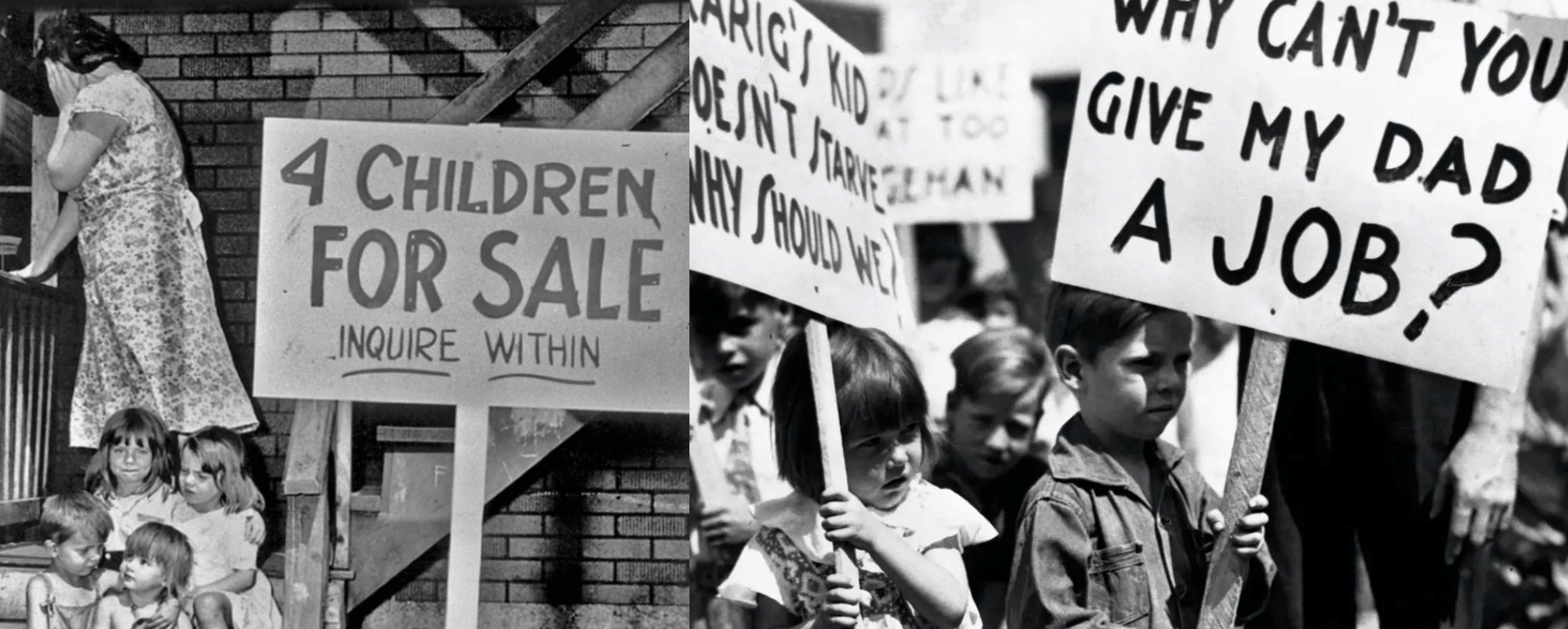
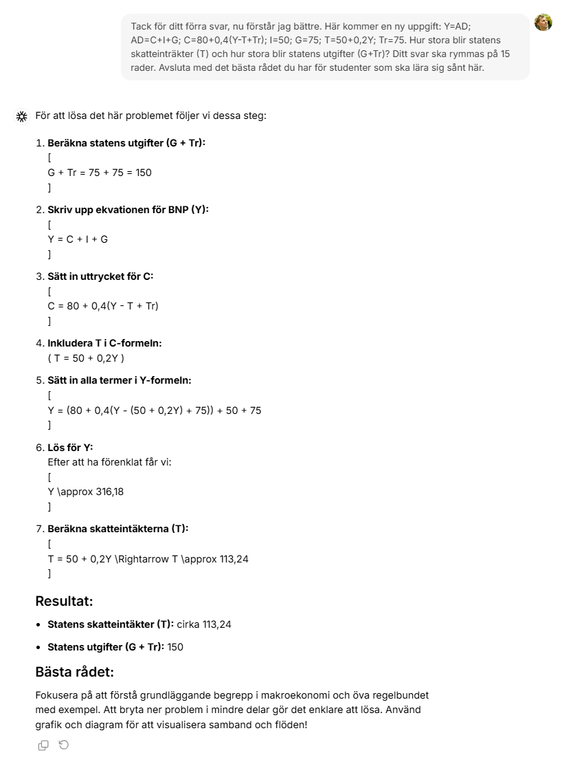
- The crisis spread across the globe. Assume you know the following about a country: \(\small Y_P=700\), \(\small AD=C+I+G\), \(\small C=70+0,8Y\), \(\small I=40\) och \(\small G=20\).. The country’s GDP in the very short run is therefore and the country is thus in .
- The GDP gap shows the percentage difference between actual GDP and potential GDP. Approximately how large is the GDP gap? Answer:
- Suddenly pessimism hits investors, causing investment to change to I = 30. The effect of this investment pessimism makes GDP in the very short run fall to .
- The multiplier for I shows how GDP changes if I increases by one unit. How large is the multiplier for I in our case? Answer: .
- The size of the multiplier in our example is determined by the marginal propensity to consume. The multiplier is larger the the marginal propensity to consume is. Make sure you understand why!
- For another country you know: \(\small C=80+0,4YD\), \(\small I=50\), \(\small G=75\), \(\small T=50+0,2Y\), \(\small Tr=75\), where YD is disposable income. Authorities report that the government deficit is just under 10 percent of GDP. Are the authorities lying? Answer: , because the deficit corresponds to almost of GDP.
- If you still struggle with these types of exercises, get help from classmates or teachers. Another option is to consult ChatGPT — but don’t trust it blindly.
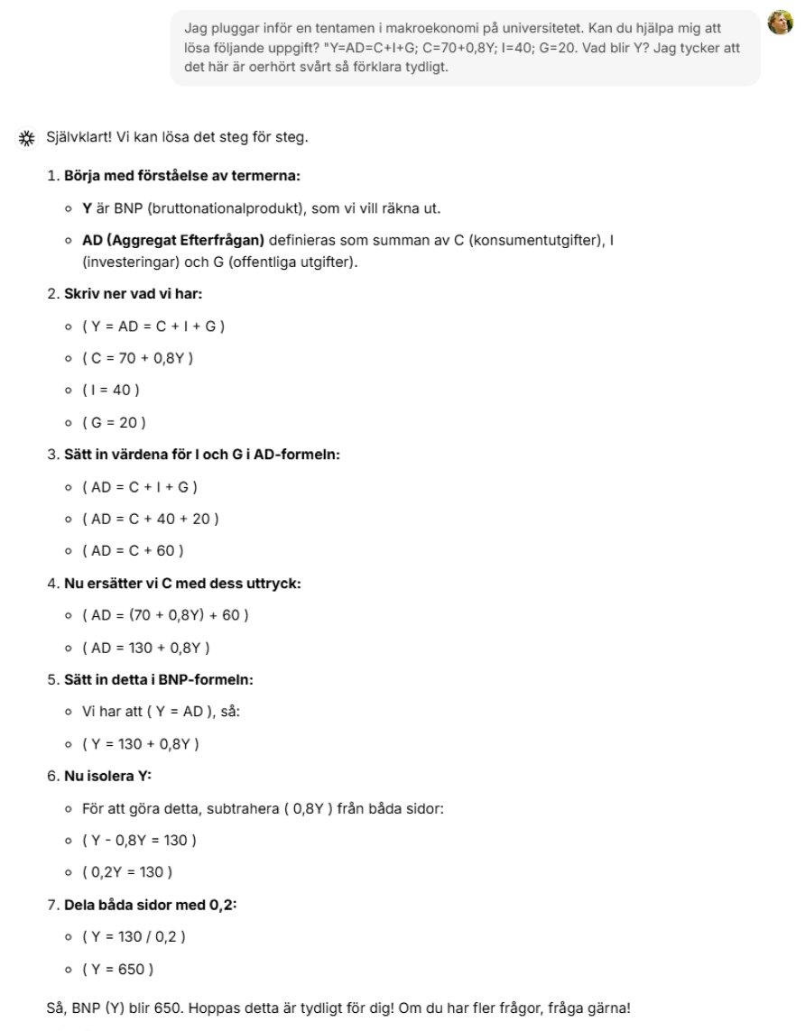
- Since actual GDP is 650 and potential GDP is 700, the country is in a recession. The GDP gap shows the distance to potential GDP (in percent). We are therefore 50 below Yp. Whether that is large or small depends on the level of Yp — being 50 below Yp is far worse if Yp = 100 than if Yp = 10,000.
- Follow the calculations in question 1 exactly, but substitute I = 30 instead of 40.
- Here you must grasp the multiplier concept. In the exercise I fell by 10 and Y fell by 50. The effect on GDP was therefore 5 times larger than the initial change in AD. The multiplier is thus 5. Make sure you understand what this means, for example if you consider using discretionary fiscal policy to pull Finland out of a recession. By the way, do you understand what discretionary fiscal policy means?
- Play with the app higher up in the chapter until you understand how it works. Also look at the circular‑flow diagram and think about what happens when I suddenly increases.
- As always: collaborate with others — don’t isolate yourself! People are best, but ChatGPT can also be useful.
Combating an economic crisis
With the help of government economic policy it is possible to influence the macroeconomy, but steering a country’s GDP is like steering a gigantic ship. You must know exactly where you are and where you want to go — and to avoid running aground you must turn in good time and steer just the right amount.
- “The idiot in the shower” is a term used to describe .
- Assume income up to EUR 10,000 is taxed at 10%, income between EUR 10,000 and EUR 40,000 is taxed at 40%, and all income above that is taxed at 90%. You earn EUR 20,000. Your marginal tax rate is therefore and you pay of your income in tax.
- The tax system in question 2 above is an example of a tax system.
- In fiscal policy people talk about the three Ts: timely, temporary, targeted. Explain in simple words the difference between discretionary fiscal policy and automatic stabilisers. Define the terms first and relate your answer to the three Ts.
- Good news, right? Your study grant rises from EUR 280 to EUR 308! At the same time the CPI rises from 140 to 161. How is your purchasing power affected? Answer: .
- Bad news, then? Your monthly salary is cut from EUR 6,000 to EUR 5,700. At the same time the CPI falls from 200 to 188. How is your purchasing power affected? Answer: .
- Read the chapter.
- Here you must understand the difference between the marginal tax rate and the average tax rate.
- Read the chapter.
- My tip for this kind of question is to write your answer on paper now. Then read it aloud to yourself or — even better — to a classmate. Did the answer have depth? Can the reader understand what you say? Can you improve it before the exam?
- Your nominal grant rises by 10% while prices rise by 15% — so your real income falls by 5%.
- Your monthly wage was cut by 5% while prices fell by 6% — so your purchasing power has increased by 1%.
Are there political business cycles?
This map shows what the border area between Sweden and Finland looks like up in the Bay of Bothnia. On the left you can see Haparanda, on the right Tornio.

- In your bachelor thesis you want to investigate whether there are political business cycles in Sweden. Explain the concept political business cycles in plain language.
- Use the AD‑AS model to explain how a political business cycle arises. Make sure your figure is neat: clearly label the axes, identify each curve, show the initial equilibrium and then what happens.
- One way to test for political business cycles is to check whether municipalities tend to cut local income taxes in election years. The municipal tax rates for every Swedish municipality 2000–2024 are available here. For example, select Total municipal tax rate, choose Municipalities, find and mark Haparanda, tick all years and press Continue. Haparanda held municipal elections in 2002, 2006, 2010, 2014, 2018 and 2022. Do you see any sign in the data that Haparanda’s politicians use tax cuts to win votes in election years?
- The raw data may show no clear tax cuts in Haparanda in election years — but how do you know what would have happened to Haparanda’s tax rate had there not been an election? Other events (e.g. the pandemic in 2022) may have prevented tax cuts. One solution is to compare what happened in municipalities that did not hold elections that year (for example Tornio, just across the border). Dahlberg & Mörk (2008) studies political business cycles by comparing all Swedish and Finnish municipalities and finds: “in an election year municipal employment and municipal consumption are higher than in a non‑election year, while the tax rate is not as high.” Do you think budgets should be legally required to balance in order to prevent local politicians abusing fiscal policy for re‑election? What are the pros and cons of that proposal?
- Read the chapter and write your answer on paper. Read it aloud! Is the answer spot‑on or can it be improved?
- Start from, for example, point 1 in Figure 14.6. Then show what happens in the short run with expansionary fiscal policy. The figure must of course be crystal clear and your explanation coherent and well informed. Try to demonstrate that you have studied the material thoroughly!
- You may not see clear signs in Haparanda that politicians cut taxes in election years. If you write a longer economics paper (and master quantitative methods) you can download data for all municipalities and investigate the question more professionally. You will take courses like that if you continue with economics. Important: put in the work.
- Banning politicians from using the tax lever can stop abuse of power (good!) but also prevents using fiscal policy to fight crises (bad!). As always, there are pros and cons.
- If you want to learn more about public debt in Europe see here.
- The 2008 financial crisis threw the world into a deep recession. This film explains why the crisis occurred — and how it was fought using, among other things, expansionary fiscal policy: