19 We are the world
(where you learn how globalisation affects your life)
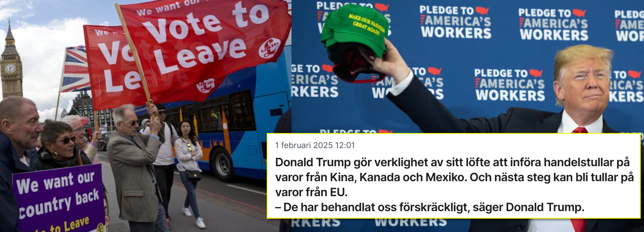
A key lesson in this book has been that we gain from cooperating with others. In the Adam and Eve example in Figure 2.2 we saw how both could go home earlier by dividing tasks. By specialising in their comparative advantages they became more efficient. Likewise, people in Turku can be better off by trading goods and services with neighbours in Helsinki — very few think Turku’s prosperity depends on building a wall around the city. Yet when it comes to international trade many reason differently. For example, President Trump has long threatened higher tariffs to restrict trade with the EU, China and Mexico.

It’s time for us to study globalisation and its effects. Is Trump right in his criticism of globalisation? For example, is it true that the highly educated gain from globalisation while low‑skilled jobs disappear or move abroad? That is the theme of this chapter.
19.1 Finland in the world
This map shows how important international trade was for different countries in 2025. It sums each country’s exports — what they sell to the rest of the world — and imports — what they buy from abroad. That sum is then related to the country’s GDP, giving a picture of how trade‑dependent a country is.
Finland’s figure was 83.4%. That means the sum of our exports and imports corresponds to 83.4% of GDP. Just over 40% of everything we consume in Finland is manufactured abroad, and roughly the same share of our domestic production is exported to other countries. As the map shows, international trade is extremely important for most countries — typically more important for small nations than for large ones. Understanding our trade with the world is therefore crucial if you want to understand life in Åbo.
globalisation is when the world’s economies become more interconnected, making it easier for goods, services, people and capital to move across borders
free trade exists when trade between countries is not restricted by tariffs or other trade barriers
protectionism refers to measures aimed at shielding the domestic sector from foreign competition, for example through tariffs or import restrictions
If you click any country on the map you can follow its trade over time. In most countries the curves slope upward: trade with other nations has become more important almost everywhere. Over time the world’s countries have grown increasingly intertwined. But why has the world opened up for you while your grandmother could only cooperate with people in her village? One key explanation is new technology. Technological progress has made it far cheaper to communicate and transport goods over long distances. The following figure shows how transport and communication costs have collapsed since 1930:
But the world has also become more open because of political reforms. More and more countries have realised that openness to the outside world is good for the economy. The same principle that applied to Adam and Eve can also be applied to countries. What do you make of the following figure?
On the horizontal axis you see each country’s average economic growth since 1945. For example, South Korea’s economy has grown by almost 6 percent per year on average, while North Korea’s GDP has fallen by more than 7 percent per year. The vertical axis shows what happened to openness, here measured as exports’ share of GDP. South Korea has on average become more than 5 percentage points more open each year since 1945, while North Korea has on average become almost 17 percentage points more closed each year. Click Select countries and regions if you want to find Finland in the chart quickly.
If you drew a line that best describes the relationship between openness and growth, it would slope upward, right? There are exceptions, of course, but many of the countries with the highest economic growth since 1945 are precisely those that opened up most to international trade. Isolation has rarely been a path to prosperity. This pattern shows how important it is for countries to be open to international trade.
With WHOM do we trade?
Now let’s examine Finland’s actual trade with the world. Here I’ve made a figure showing Finland’s exports to each country in 2024:
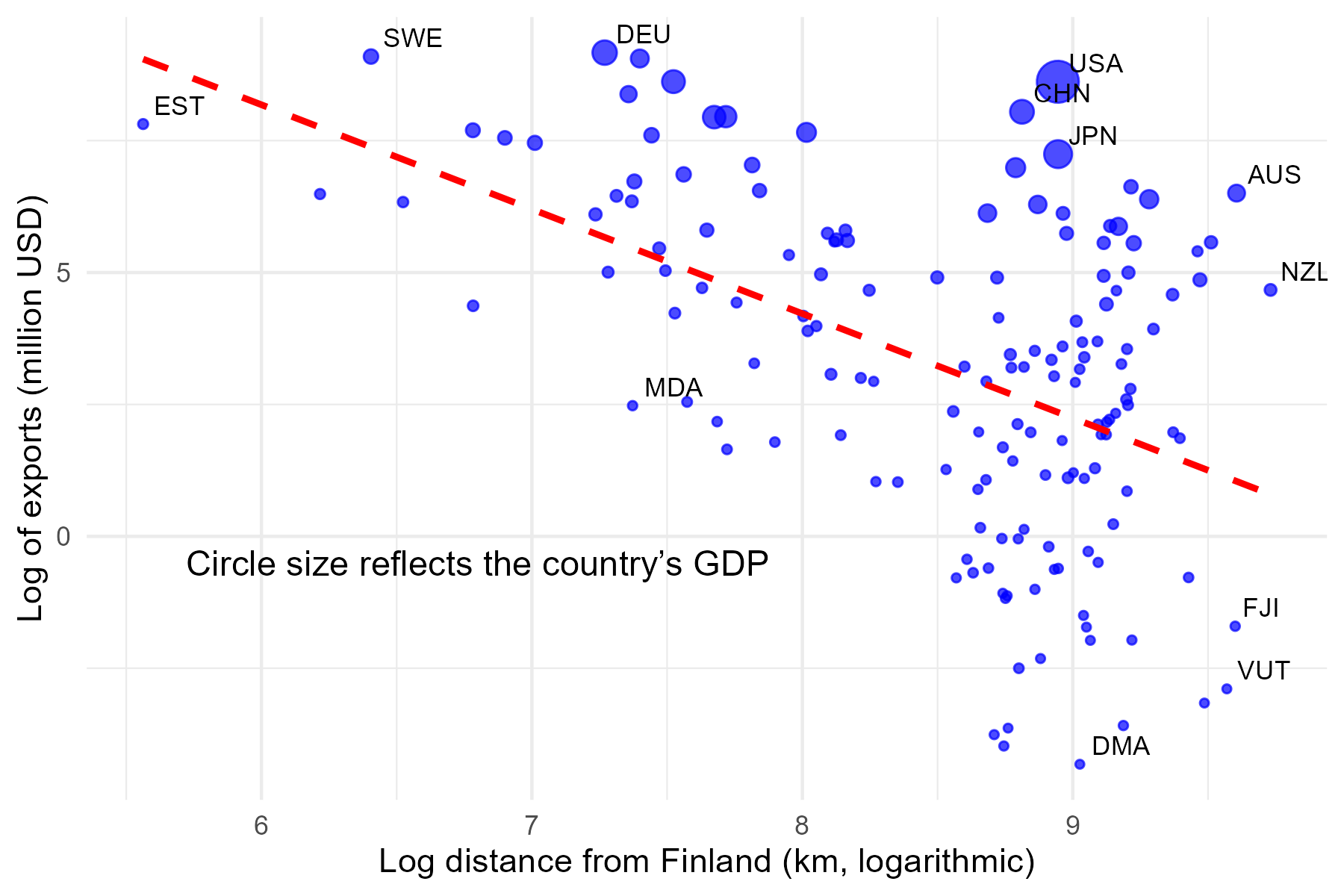
The horizontal axis in the chart shows the distance from Finland to each country, while the vertical axis represents how much Finland exported to those countries. Each circle is a country, and the circle size reflects the country’s GDP. What can you learn about our trade from the figure?
Distance matters: The dashed red line indicates a clear pattern. Finland tends to trade much more with nearby countries, like Estonia (EST) and Sweden (SWE). Our trade with distant countries, such as Fiji (FJI) and Australia (AUS), is much smaller. This shows that distance remains an important factor in understanding world trade.
Size matters: Do you notice that countries with large GDPs are often above the dashed line? This means Finland exports “extra” much to economically large countries. For example, we trade a lot with the USA and Japan despite the long distances.
That both distance and size are decisive for trade is reminiscent of Isaac Newton’s discovery of gravity. The gravitational pull between two bodies depends on both their masses and the distance between them; the attraction between two large planets 1 kilometre apart is far greater than between two grains of sand separated by millions of light‑years. The hypothesis that trade between countries depends on their economic size (GDP) and the distance between them is therefore called the gravity model. The figure above suggests this simple model can explain a substantial part of world trade.

What do we trade?
The gravity model predicts Finland will trade heavily with Germany and Sweden — and also with the USA and China. The next question is: what exactly do we export? The answer is shown here:
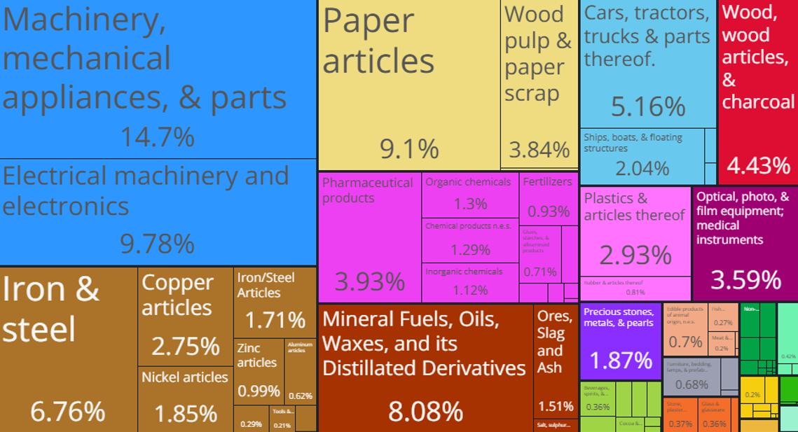
Finland exports a lot of paper, timber and advanced technical machinery. Soon we will explore why these are the products we’ve specialised in and how this trade affects us. Before we dive into trade theory it’s useful to get an intuitive feel for the subject. Watch the following introduction to international trade by Klas Eklund, a brilliant economist and lecturer.
19.2 Trade theory for beginners
In this section we will understand why our trade with the world looks the way it does, and how it affects different groups in Finland. Let us aim to understand three things:
- Why does Finland export paper and luxury yachts but import meat and toys?
- Which groups in Finland win and which lose from globalisation?
- Why does President Trump want to restrict US trade with the rest of the world?
Trade based on comparative advantage
Let us start by analysing trade between Finland and Argentina. In 2024 Finland exported goods and services to Argentina worth USD 163 million, much of it advanced technical equipment such as medical instruments. At the same time we imported goods from Argentina for USD 26.4 million, including wine for USD 3.2 million, nuts for USD 2.2 million and horsemeat for USD 1.9 million. But why does our trade with Argentina look like this?
Om du på egen hand vill lära dig mer om Finlands utrikeshandel kan du utforska data här.
Adam Smith, nationalekonomins fader, förklarade internationell handel med följande liknelse:
It is the maxim of every prudent master of a family, never to attempt to make at home what it will cost more to make than to buy. The tailor does not attempt to make his own shoes, but buys them from the shoemaker. What is prudence in the conduct of every private family can scarce be folly in that of a great kingdom. If a foreign country can supply us with a commodity cheaper than we ourselves can make it, better buy it of them with some part of the product of our own industry, employed in a way in which we have some advantage.
- Adam Smith 1776, ur “Wealth of Nations”
This is the same principle that explains why Adam and Eve could achieve more by helping each other according to their comparative advantages than by isolating themselves. Finland is “especially” good at producing advanced technical equipment, while Argentina is “especially” skilled at producing wine, nuts and horsemeat.
But why do we have a comparative advantage in advanced technology and Argentina in agricultural products? Because production always requires resources — skilled and unskilled workers, capital and land. The mix of these resources differs across countries according to their unique endowments. Compared with many others, Finland has a very highly educated population, which makes us strong in producing goods and services that require specialised labour. Likewise, Argentina has vast fertile land that is well suited to producing wine, nuts and horsemeat.

Globalisation therefore changes what we produce in Finland. We no longer need to make much wine, nuts or horsemeat ourselves; instead we can import these products from Argentina, which—thanks to its vast fertile plains—can produce them much more cheaply. That is bad news for Finnish wine producers. On the other hand, Finland’s advanced sector will grow because of globalisation. Compared with many countries we have lots of highly educated people who are crucial when producing, for example, medical instruments for cancer diagnostics. That is good news for you if you are (about to be) highly educated. Globalisation opens growing demand not only for domestic consumption but also for exports to international markets. Expect more jobs and substantial wage increases in the advanced sector!
This simple theory of international trade—the Heckscher–Ohlin model—can be used both to understand world trade and to analyse critiques of globalisation.
Why protectionism?
Trade with the rest of the world thus makes a country richer, but globalisation can also be painful for certain groups. Adermon & Gustavsson (2015) has examined which jobs have increased and which have declined over recent decades.
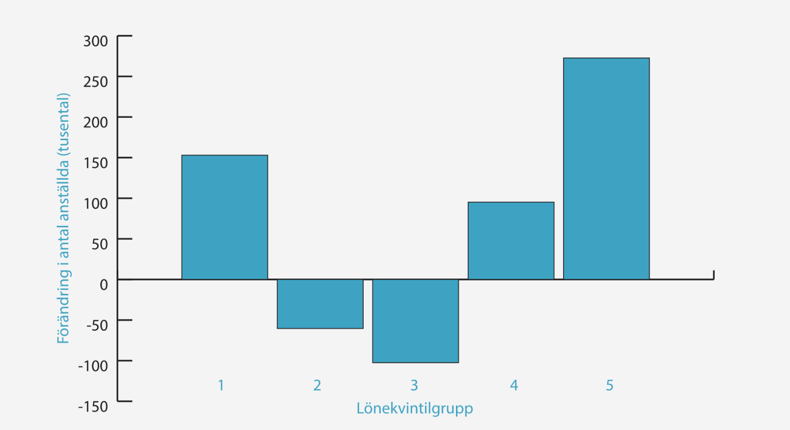
The researchers first divided all occupations into five equally sized groups based on 1975 wages. Wage‑quintile 1 includes the lowest‑paid jobs (e.g. hairdressers and cleaners), while quintile 5 contains the highest‑paid jobs (e.g. surgeons and economists). The vertical axis shows the change in the number of people working in these occupations today compared with 1975. You can see that low‑paid and high‑paid jobs have increased, while jobs in the middle segment have declined. This suggests the labour market has polarised and income gaps have widened.
Globalisation is likely an important reason why “middle jobs”, such as routine manufacturing roles, have declined. According to trade theory, if Finland’s comparative advantage lies in advanced, highly skilled activities, those jobs will expand here while simpler tasks are partly relocated abroad. Middle‑skill jobs have also been squeezed hard by new technology. Displaced workers therefore need to move into growing sectors. In short, both globalisation and technology drive a structural transformation that makes Finland richer overall but can be very painful for those who lose their jobs. Perhaps that is the root of much criticism of globalisation — what do you think?
Trade based on specialisation and economies of scale
The Heckscher–Ohlin trade theory explains trade between countries that are different. We import toys from China because China has hundreds of millions of low‑skilled workers, making it cheaper to manufacture toys there than in Finland.
But how do we understand trade between similar countries, for example Finland and Sweden? I have lived a long time in both countries and can honestly say it is practically impossible to tell them apart. So let’s look more closely at trade between Finland and Sweden. In 2024 Finland exported spirits to Sweden worth USD 17.8 million, but we also imported spirits from Sweden worth USD 3.3 million. Strange, right? Part of the spirits trade goes both ways. How can this so‑called two‑way trade arise, and what are its effects?
Think of it this way: not all spirits taste the same. An Absolut Citron is very different from a Finnish schnapps like Jaloviina. The good “spirits” is therefore differentiated. Some consumers prefer the lemony Swedish spirit, others the spicier Finnish schnapps. International trade allows the Swedish firm to produce Absolut Citron for consumers in both Sweden and Finland who like lemony spirits. This raises production volumes, which can make each bottle cheaper to produce. Economies of scale mean that larger output lowers average production costs. Likewise, the Finnish firm making Jaloviina can serve customers in both Finland and Sweden and thus cut its prices.

This kind of international trade does not have the clear losers that trade based on comparative advantage can create. Who loses if Finland exports Oltermanni cheese to Sweden and imports Grevé? Both firms benefit from larger markets, and cheese consumers in both countries get cheaper and more varied choices.
International trade is a huge and exciting field. Right now, for example, third‑year economics students in Åbo are measuring to what extent rising income inequality in rich countries is actually due to globalisation.
19.3 Currencies and exchange rates
There are other things you must know in the age of globalisation. What do you do, for example, if your boss asks you to compare what foreign PR agencies charge for running an ad campaign? The Finnish agency asks €50,000, the Swedish one SEK 450,000 and the Japanese one JPY 8,000,000. Your boss wants an answer in five minutes! This is when you’re glad you learned the basics of exchange rates. You only need to remember one formula. Here it is:
\[ \small\underbrace{\text{Exchange rate}}_{\substack{\text{Price of one euro in the other currency}}} = \frac{\text{Amount of the other currency}}{\text{Amount of euros}} \]
The exchange rate thus shows how much of the other currency you must pay to buy one euro. Because there are many different currencies — euro, dollar, krona, yen, etc. — there are also many different exchange rates. Each exchange rate shows how much of the other currency you must give up to get one euro. The list below shows the value of the euro when I write this at 16:38 on 12 February 2026.
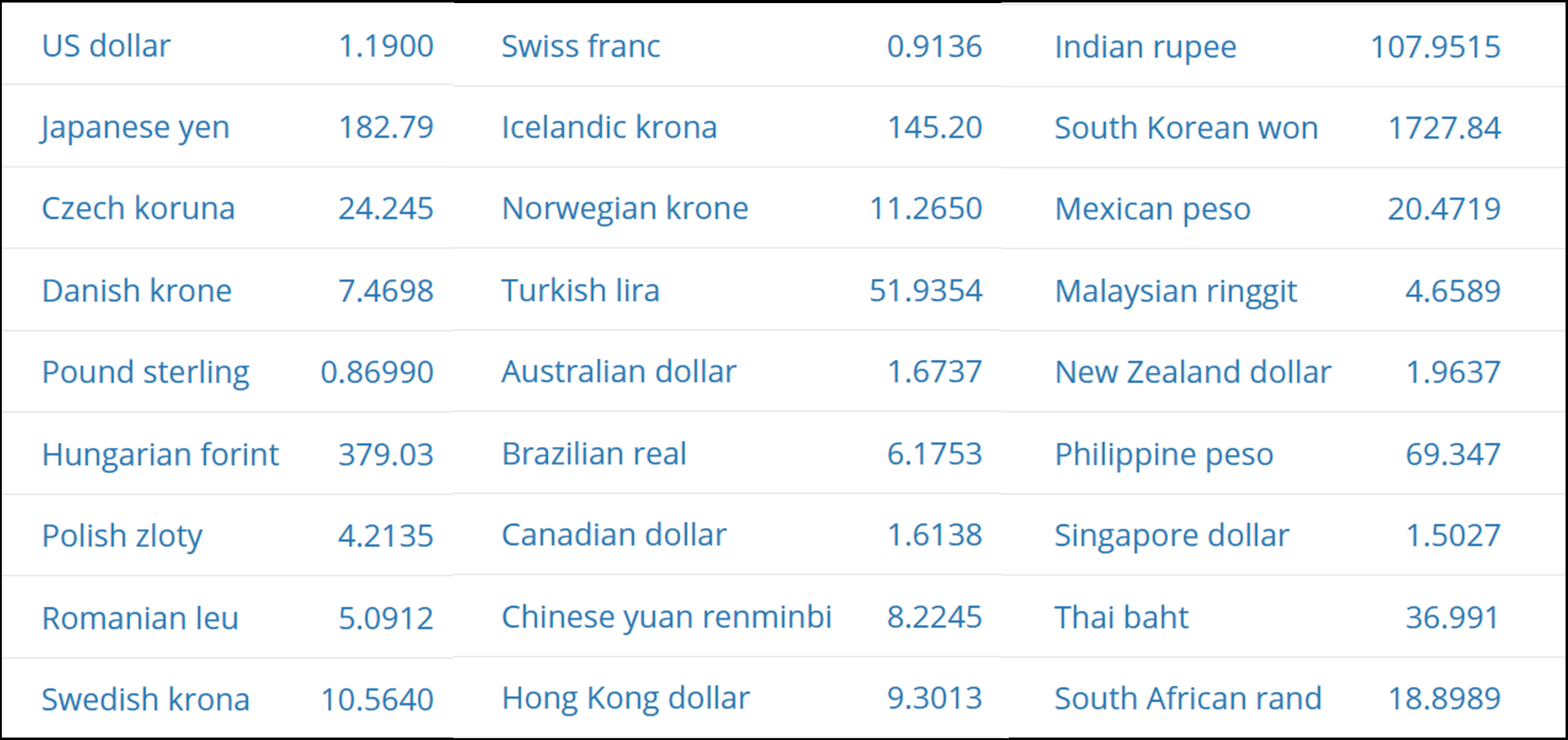
As you can see, a Swede must pay 10.564 kronor to buy one euro, an American 1.19 dollars and a Japanese resident 182.79 yen. These exchange rates change every second, and you will soon see why. The simple answer is that the foreign‑exchange market works like any other market: what many people want tends to be expensive.
The nice thing about the formula above is that you can use it to see what things cost in different currencies. For example, if you want to compare prices in Finland and Sweden you can rewrite the expression so that it becomes:
\[ \small{\text{Amount of euros}} = \frac{\text{Amount of kronor}}{\text{Exchange rate (i.e. the price of one euro in kronor)}} \]
\[ \small{\text{Amount of kronor}} = {\text{Amount of euros x Exchange rate (i.e. the price of one euro in kronor)}} \]
The Swedish agency charged SEK 450,000. Using the formula above you can see that SEK 450,000 corresponds to about EUR 42,598. Similarly, JPY 8,000,000 is roughly EUR 43,766. Assuming the agencies are equally good, it is therefore economically most advantageous to hire the Swedish firm.
When Swedes later visit Åbo and ask what a €3.40 cappuccino is in kronor you can use the inverse formula to tell them that €3.40 equals SEK 35.92.
The exchange rate affects your contacts with the rest of the world
Look at this figure showing how the value of the euro (expressed in kronor) has evolved since the euro was created in 1999.
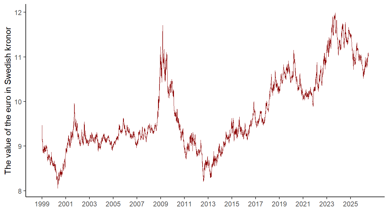
Right now — Wednesday 7 July 2026 — one euro costs SEK 11.04. Imagine you’re on holiday in Stockholm and see a large beer for SEK 75. At today’s exchange rate that would cost you EUR 6.79. Remember the euro’s value affects what you pay for Swedish beer. When the euro was stronger — for example summer 2023 when one euro was almost SEK 12 — the beer effectively cost only about EUR 6.25. Compare this with 2012–2013, when the euro was worth only SEK 8 and the same beer cost EUR 9.37.
The euro’s value therefore affects how attractive it is to buy things in the other country: a strong euro gives you more kronor per euro, so it’s cheap for you to shop abroad. The opposite holds for the Swede visiting Åbo. A weak euro can also raise inflation in Finland: imported goods (like Swedish beer) become more expensive. At the same time a weak euro attracts more Swedes to travel to Åbo while Finns stay home, boosting domestic demand.
exchange rate is the price of a foreign currency relative to your own currency
EMU, the Economic and Monetary Union, was formed in the 1990s to deepen economic cooperation within the EU; all EU countries are part of the EMU framework but not all use the euro
What determines the value of one euro?
But why does the price of the euro change? The simple answer is that a currency is like any other good: when demand for it rises its price usually goes up. When people suddenly go crazy for sushi or central‑Helsinki apartments those prices rise — the euro market works the same way.
Who shows up at the market to buy and sell euros — and what drives their decisions? Think of the market as a foreign‑exchange kiosk. Finns come to exchange their euros for Swedish kronor — maybe you preparing for a weekend in Stockholm, needing kronor for cafés and taxis, or you hiring a Swedish PR firm, or choosing to save in a Swedish bank. But people who want euros also come to the kiosk: Swedes (and others) who need euros to buy and invest in Finland. You can picture the FX market looking roughly like this:
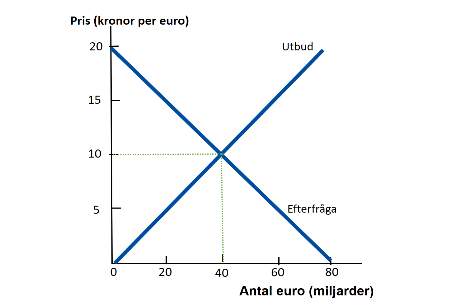
The supply shows how many euros sellers (you) want to sell and demand shows how many euros buyers (me) want to buy. Do you see why the supply curve slopes up? Remember that a strong euro means you get many kronor in exchange for each euro. That gives you lots of money for your Stockholm trip. Because it’s cheap in Stockholm more Finns will find a Sweden holiday attractive, so the stronger the euro, the more Finns will want to sell their euros.
Do you likewise see why the demand curve slopes down? A strong euro makes it expensive for Swedes to do things in Finland. The weaker the euro becomes, the more Swedes will want to visit Finland — so Swedes demand more euros when the euro is cheap. You can imagine Swedes need to give up fewer kronor to buy one euro. Market forces push the euro price in Figure 19.4 to, say, 10 kronor because only at that price do buyers want to buy exactly as many euros as sellers want to sell. If the price were 15 kronor per euro there would be many more Finns wanting to sell euros than Swedes wanting to buy, so sellers would have to accept a lower price. If the price were below equilibrium — say 5 kronor per euro — lots of Swedes would want euros but very few Finns would sell at that poor price; Swedes would need to offer a better price to convince Finns to sell.
Shocks and the euro’s value
If you understand the basics of how a market works you can also see why the euro’s price changes. Consider these two shocks. What happens to the euro price expressed in kronor?
Case 1: Finland becomes a model country. Suddenly the world is amazed: Finland is the best country — everything works! The economy booms; Finns are extremely innovative and new inventions appear every day. People want Finnish goods and services, and foreigners may want to move their savings into Finnish banks or buy Finnish stocks. Currency analysis: this raises demand for euros — the demand curve shifts right. Supply will also react: fewer Finns want to sell euros if Finland becomes a dream destination, so the supply curve shifts left. The net effect is that the euro appreciates.
Case 2: Political collapse in the EMU area. The unthinkable happens: many countries have huge public debts after years of living beyond their means. Politicians say they won’t repay debts and some observers fear the survival of democracy. Currency analysis: would you want to move there or invest there? Probably not. Instead people look elsewhere (e.g. the US). More people try to sell euros (supply shifts right) while fewer want to buy them (demand shifts left). The euro depreciates.
Your own currency forecast
Is it possible to predict a currency’s path? Let’s go back in time to test it! The euro’s value (in other currencies) on 12 February 2025 is shown here. At the start of 2025 one euro therefore cost SEK 11.25. The image below shows what a Big Mac cost on the same day in Haparanda (Sweden) and in Tornio (Finland).

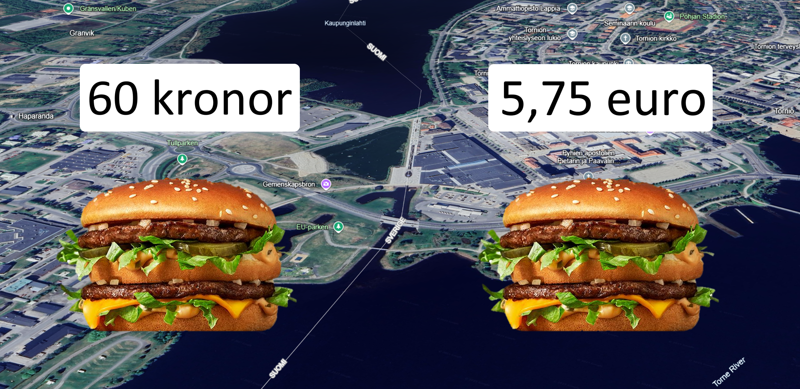
Do this thought experiment: You’re in Tornio on 12 February 2025. You have €5.75 in your pocket — enough to buy exactly one Big Mac in Tornio. But what if you buy the Big Mac in Haparanda instead? You’d first need to convert your euros into Swedish kronor. At an exchange rate of SEK 11.25 per euro you get almost SEK 65 for your €5.75. With SEK 65 in your pocket you walk into a McDonald’s in Sweden and find, to your surprise, that the money more than covers the price — you even have change left over. Apparently a Big Mac was cheaper in Sweden than in Finland in early February 2025.
What does this imply for the euro? The situation suggests it’s more attractive to shop in Sweden than in Finland. Over time more people should notice this, which would lead more Finns to sell euros while fewer Swedes want euros. That should cause the euro to weaken against the krona. This simple analysis suggests the euro was overvalued against the krona in early 2025 and therefore likely to fall in value (meaning the krona should strengthen). Want to check whether your forecast was right? See the current euro rate here. Based on your analysis, is the euro currently “fairly” valued or do you expect it to go up or down?
Is the euro good or bad for Finland?
Whether it was a good decision for Finland to join the euro is still contested. Sweden chose to keep the krona. Who was right? In theory there are mainly two advantages and two disadvantages of a common currency:
Advantage 1: Facilitates international trade. A common currency makes trade easier. You no longer need to worry about exchange‑rates. That simplifies cooperation and commerce. And we’ve said cooperation benefits everyone. So the euro is good!
Advantage 2: A straitjacket that forces good policy. Imagine a small country that gets everything wrong: schools fail, universities are a joke, corruption is rampant, inflation is high, innovation is scarce, policy is incompetent and the country’s goods and services are poor. Such a country would struggle to compete. Its currency would depreciate, however, and that depreciation would make exports a bit easier (think about what a Swede pays for a cappuccino in Åbo if the euro weakens). The loss of competitiveness that comes with a weakening currency can force politicians to tackle the country’s real problems. Finland’s competitiveness within the euro area can only be improved by making fundamental reforms at home.
Disadvantage 1: Does a single monetary policy suit the entire EMU? With the euro monetary policy is common to all EMU countries. Today Christine Lagarde and her colleagues at the ECB in Frankfurt decide whether policy should be loose or tight. But does the same policy suit every country? Imagine Finland is in recession while the rest of Europe is booming. Lagarde may raise rates to prevent overheating — good for most of Europe, but a disaster for Finland. That is why countries adopting a common currency should be fairly similar; economists talk of an optimal currency area. The more heterogeneous the countries, the greater the risk that a single monetary policy will be inappropriate for some members.
Disadvantage 2: You can no longer be rescued by a weaker currency. Advantage 2 can also be framed as a drawback. Suppose a fungus wipes out nearly all spruces in the Nordics. The krona would weaken and that would help Sweden’s exports. Finland, however, is so small relative to the entire euro area that what happens there has almost no effect on the euro’s value. A depreciating euro will not rescue Finland in the same way a weaker krona could. The shock would therefore hit Finland harder than it would a standalone Sweden.
19.4 Business‑cycle analysis for pros
So far our business‑cycle analysis has ignored the rest of the world. For example, we treated aggregate demand as coming only from Finnish households’ consumption (C), Finnish firms’ investment (I) and government consumption (G). A professional analysis must of course also account for what happens abroad. For example, GDP in China and India has grown by nearly 10 percent per year during your lifetime. That means 2.7 billion Chinese and Indians have become substantially richer, and some of their extra income will likely be spent on goods and services from Finland.
If you understand how to analyse a closed economy, it is relatively straightforward to extend the framework to an open economy. The only thing you need to do is think of the circular flow of the economy — but with a twist:
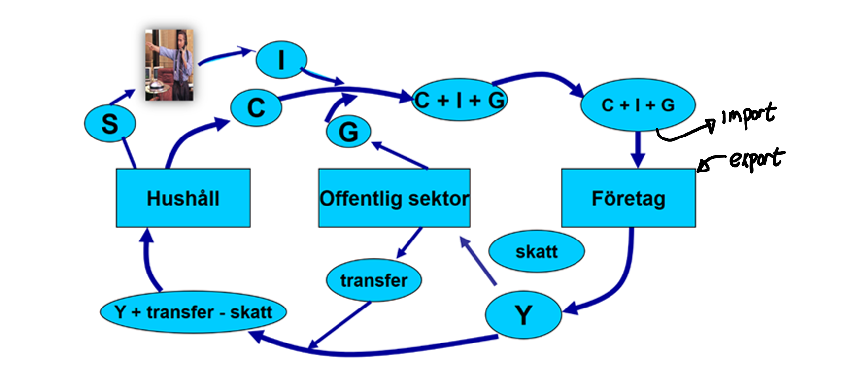
What’s different from before? Imagine you run a small bicycle company in Turku. It’s perfectly possible that people abroad want to buy your bikes — so we must add all demand directed at Finnish firms that comes from abroad. Likewise, Finnish households that want to buy bikes may choose to buy them in Sweden instead — so we must subtract all demand in Finland that goes to foreign firms. In the very short run GDP is determined by total demand, which in an open economy looks like this:
\[ \small\text{Y = AD = C + I + G + EXPORT - IMPORT} \]
As soon as the rest of the world wants more of Finland (for example because their households feel richer or because their firms want to invest in new cruise ships and therefore hire Åbo shipyard Meyer Turku), AD in Finland rises and our GDP increases in the short run. Likewise, a financial crisis in the USA will pull Finland’s economy down.
At the end of the chapter there are exercises where you practise business‑cycle analysis in an open economy. Below I’ve also made an app you can play with if you’re interested. Note that models can always be made more or less realistic.
#| standalone: true
#| viewerHeight: 1650

if (!requireNamespace("shiny", quietly = TRUE)) install.packages("shiny")
if (!requireNamespace("plotly", quietly = TRUE)) install.packages("plotly")
if (!requireNamespace("grid", quietly = TRUE)) install.packages("grid")
if (!requireNamespace("scales", quietly = TRUE)) install.packages("scales")

library(shiny)
library(plotly)
library(grid)
library(scales)

safe_numeric <- function(x, default = 0) {
  if (is.null(x) || identical(x, "") || is.na(as.numeric(x))) return(default)
  as.numeric(x)
}

# Helper for consistent formatting
fmt <- function(x) comma(x, accuracy = 0.01, decimal.mark = ".", big.mark = ",")

ui <- fluidPage(
  fluidRow(
    column(width = 4,
      wellPanel(
        numericInput("a", "Autonomous consumption (a):", value = 100, min = 0, step = 1),
        numericInput("b", "Marginal propensity to consume (b):", value = 0.8, min = 0, max = 0.99, step = 0.01),
        numericInput("I", "Investment (I):", value = 50, min = 0, step = 1),
        numericInput("G", "Government spending (G):", value = 80, min = 0, step = 1),
        numericInput("c", "Autonomous tax (c):", value = 10, min = 0, step = 1),
        numericInput("d", "Marginal tax rate (d):", value = 0.4, min = 0, max = 0.99, step = 0.01),
        numericInput("Tr", "Transfers (Tr):", value = 80, min = 0, step = 1),
        numericInput("EXP", "Exports (EXP):", value = 20, min = 0, step = 1),
        numericInput("p", "Autonomous imports (p):", value = 10, min = 0, step = 1),
        numericInput("q", "Marginal propensity to import (q):", value = 0.1, min = 0, max = 0.99, step = 0.01),
        numericInput("maxY", "Max value for output (Y) in the figure:", value = 800, min = 10, step = 10),
        actionButton("calculate", "Calculate and illustrate!",
                     style = "color: white; background-color: #007bff; padding: 6px 12px; border: 2px solid #007bff;"),
        br(),
        tags$small("Model: C = a + b(Y - T + Tr); T = c + dY; IMP = p + q·Y. Click 'Calculate and illustrate!' to update.")
      )
    ),
    column(width = 8,
      plotlyOutput("adAsPlot"),
      br(),
      verbatimTextOutput("equilibriumOutput")
    )
  )
)

server <- function(input, output, session) {

  validate_params <- function(a, b, c, d, I, G, Tr, EXP, p, q, maxY) {
    if (any(is.na(c(a, b, c, d, I, G, Tr, EXP, p, q, maxY)))) return("Error: Please provide all parameters.")
    if (b < 0 || b >= 1) return("Error: b must be in [0, 1).")
    if (d < 0 || d >= 1) return("Error: d must be in [0, 1).")
    if (q < 0 || q >= 1) return("Error: q must be in [0, 1).")
    if (maxY <= 0) return("Error: maxY must be greater than 0.")
    NULL
  }

  observeEvent(input$calculate, {
    a <- safe_numeric(input$a)
    b <- safe_numeric(input$b)
    c <- safe_numeric(input$c)
    d <- safe_numeric(input$d)
    I <- safe_numeric(input$I)
    G <- safe_numeric(input$G)
    Tr <- safe_numeric(input$Tr)
    EXP <- safe_numeric(input$EXP)
    p <- safe_numeric(input$p)
    q <- safe_numeric(input$q)
    maxY <- max(10, safe_numeric(input$maxY))

    err <- validate_params(a, b, c, d, I, G, Tr, EXP, p, q, maxY)
    if (!is.null(err)) {
      showNotification(err, type = "error")
      output$equilibriumOutput <- renderText({ "" })
      output$adAsPlot <- renderPlotly({ NULL })
      return()
    }

    # Analytical equilibrium
    denom <- 1 - (b * (1 - d) - q)
    if (abs(denom) < .Machine$double.eps^0.5) {
      Y_e <- NA_real_
    } else {
      numer <- a - b * c + b * Tr + I + G + EXP - p
      Y_e <- numer / denom
    }
    if (!is.finite(Y_e)) Y_e <- NA_real_

    # Public finances and trade
    T_e <- c + d * (ifelse(is.na(Y_e), 0, Y_e))
    public_spending <- G + Tr
    public_result <- T_e - public_spending
    budget_balance_pct <- ifelse(is.na(Y_e) || Y_e == 0, NA_real_, (public_result / Y_e) * 100)

    C_e <- a + b * (ifelse(is.na(Y_e), 0, Y_e) - (c + d * ifelse(is.na(Y_e), 0, Y_e)) + Tr)
    IMP_e <- p + q * (ifelse(is.na(Y_e), 0, Y_e))
    net_trade <- EXP - IMP_e
    total_AD_at_Ye <- C_e + I + G + EXP - IMP_e

    output$equilibriumOutput <- renderText({
      if (is.na(Y_e)) {
        "No well-defined equilibrium (parameters lead to a degenerate result)."
      } else {
        paste0(
          "Facts about the equilibrium:\n",
          "Output (Y*): ", fmt(round(Y_e, 2)), "\n",
          "Consumption (C): ", fmt(round(C_e, 2)), "\n",
          "Investment (I): ", fmt(round(I, 2)), "\n",
          "Government spending (G): ", fmt(round(G, 2)), "\n",
          "Exports (EXP): ", fmt(round(EXP, 2)), "\n",
          "Autonomous imports (p): ", fmt(round(p, 2)), "\n",
          "Marginal propensity to import (q): ", fmt(round(q, 3)), "\n",
          "Imports at Y*: ", fmt(round(IMP_e, 2)), "\n",
          "Net trade (EXP - IMP): ", fmt(round(net_trade, 2)), "\n",
          "Total AD at Y*: ", fmt(round(total_AD_at_Ye, 2)), "\n",
          "Tax revenue (T): ", fmt(round(T_e, 2)), "\n",
          "Public result (T - G - Tr): ", fmt(round(public_result, 2)), "\n",
          "Budget balance (% of Y): ", ifelse(is.na(budget_balance_pct), "NA", paste0(fmt(round(budget_balance_pct, 2)), "%"))
        )
      }
    })

    output$adAsPlot <- renderPlotly({
      Y_range <- seq(0, maxY, length.out = 500)
      AD_values <- a + b * (Y_range - (c + d * Y_range) + Tr) + I + G + EXP - (p + q * Y_range)
      AS_values <- Y_range

      p <- plot_ly() %>%
        add_lines(x = Y_range, y = AD_values, name = "AD (C + I + G + EXP - IMP)",
                  line = list(color = "darkred"), hoverinfo = "text",
                  text = ~paste0("Y=", round(Y_range,1), "<br>AD=", round(AD_values,2))) %>%
        add_lines(x = Y_range, y = AS_values, name = "45° (Y)",
                  line = list(color = "black", dash = "dash"), hoverinfo = "text",
                  text = ~paste0("Y=", round(Y_range,1)))

      # Mark equilibrium with dashed lines and a point (point not in legend)
      if (!is.na(Y_e) && is.finite(Y_e) && Y_e >= 0 && Y_e <= maxY) {
        p <- p %>%
          add_segments(x = Y_e, xend = Y_e, y = 0, yend = Y_e,
                       line = list(color = "green", dash = "dash"), showlegend = FALSE) %>%
          add_segments(x = 0, xend = Y_e, y = Y_e, yend = Y_e,
                       line = list(color = "green", dash = "dash"), showlegend = FALSE) %>%
          add_markers(x = Y_e, y = Y_e, marker = list(color = "green", size = 6), showlegend = FALSE,
                      hoverinfo = "text", text = paste0("Y* = ", fmt(round(Y_e,2))))
      } else if (!is.na(Y_e)) {
        p <- p %>% add_annotations(x = maxY * 0.95, y = maxY * 0.95, text = "Y* outside range", showarrow = FALSE, font = list(color = "red"))
      }

      p %>%
        layout(
          xaxis = list(title = "Output (Y)", range = c(0, maxY), tickformat = ",.0f"),
          yaxis = list(title = "Aggregate demand (AD)"),
          font = list(size = 13, family = "Arial"),
          legend = list(x = 0.78, y = 0.95, bgcolor = "rgba(255,255,255,0.95)", font = list(size = 11)),
          margin = list(l = 60, r = 20, t = 20, b = 60),
          shapes = list(
            list(type = "line", x0 = 0, x1 = 0, y0 = 0, y1 = 1, xref = "x", yref = "paper", line = list(color = "black", width = 1.2)),
            list(type = "line", x0 = 0, x1 = 1, y0 = 0, y1 = 0, xref = "paper", yref = "y", line = list(color = "black", width = 1.2))
          )
        )
    })
  })
}

shinyApp(ui = ui, server = server)
Stabilisation policy in an open economy
Earlier in the course you learned how fiscal and monetary policy are conducted. We saw that these measures can affect real variables such as GDP and unemployment in the short run, while in the long run they only affect nominal variables like prices and wages. But all that was in a closed economy. How does the picture change once we recognise that Finland is connected to the rest of the world? The interesting conclusion is the following:
Globalisation makes monetary policy more effective, but fiscal policy weaker!
Imagine what happens when Sweden’s central bank, the Riksbank, tries to stimulate Sweden with expansionary monetary policy. It cuts its policy rate, and other rates quickly follow. Lower rates have several effects in Sweden. As we know, lower rates raise C and I. But another effect now appears. With a poor return it becomes less attractive to save in Sweden. Savers start looking abroad — perhaps interest rates are higher in Finland or the US. That makes Swedes want to get rid of kronor and buy euros or dollars (needed if you want to save in a Finnish or a New York bank). The krona weakens — and a weaker krona is BINGO for Swedish exports. The net effect is that C, I and EXPORT all increase. A Riksbank rate cut therefore has a very strong impact on the country’s GDP.
Now think of Sweden’s finance minister. She also wants to stimulate the economy and therefore uses expansionary fiscal policy. What happens? In the short run the economy heats up: higher GDP and lower unemployment — but also higher interest rates because everyone wants to consume and invest in the good times. The increased demand for kronor makes the krona stronger. With a stronger krona it becomes harder for Swedish firms to sell abroad. The finance minister thus raises C and G, but her measures also push EXPORT down. In the end expansionary fiscal policy therefore has little net effect on national GDP.
Exercises
In this chapter you have learned about globalisation and world trade. You have also learned more about currencies and economic policy in a world where countries are interconnected. Below are some cases where you can apply your knowledge in practice. Press Show Answers when you want the computer to grade your responses. Good luck!
The effects of globalisation
With trade theory you can understand why countries trade with each other — and what the consequences are. This also means you can use the models to predict what will happen if protectionism rises worldwide in the coming years.
- In the age of globalisation it’s important you know a lot about the world. What happens abroad directly affects Finnish firms and the Finnish economy. So how well do you know China and India, two giant markets with almost three billion people? Can you name ONE living Chinese or Indian person? Answer: .
- The gravity model predicts that Italy likely trades with Germany than with Sweden, and that Finland likely trades with Morocco than with Spain.
- According to the Heckscher–Ohlin model trade between country A and country B arises because .
- Two‑way trade means that countries .
- Finland exports about USD 5 billion of goods and services to China each year and imports nearly USD 8 billion from China. Much of our economy therefore depends on how China performs.
- The gravity model predicts that trade volumes between two countries depend on their economic size (GDP) and the distance between them.
- Remember Heckscher–Ohlin: comparative advantages arise from differences in countries’ resource mixes. For example, producing hand‑woven carpets requires lots of low‑skilled labour and little capital, so India can make carpets cheaply — that becomes its comparative advantage.
- Note that Finland both exports spirits to Sweden and imports spirits from Sweden. This is an example of two‑way trade.
Currency analysis
Foreign‑exchange trading is bigger than most of us imagine. Every day currencies worth over USD 6 trillion are traded.

- Assume a cappuccino costs €3.40 in Åbo — what does this mean for tourists from Sweden? The euro’s value in kronor is shown in Figure 19.3. When the euro was strongest the cappuccino cost about kronor, and when the euro was weakest it cost about kronor.
- A Big Mac cost £4.59 in the UK and USD 5.79 in the US in February 2025. On the FX market one pound could be exchanged for USD 1.258. This indicates a Big Mac was in the UK than in the US, which suggests the pound was against the dollar and therefore was likely to in value in the future.
- Since 2013 the euro has strengthened against the krona. Can you explain, using economic theory, why the euro could have appreciated relative to the krona? Illustrate your reasoning with a figure of the FX market.
- In late February 2022 the Russian rouble suddenly collapsed. Why did this happen? Illustrate and explain.
- On 20 January 2025 Donald Trump was sworn in as US president. Based on economic theory, how do you think his presidency affected the dollar’s value? You can see how the dollar actually evolved (in euros per dollar) here.
- Give one economic argument for why it might have been better for Finland to keep the Finnish markka instead of adopting the euro.
- Remember: a strong euro makes it cheap for you to shop in Stockholm but expensive for me as a Swede to shop in Åbo.
- The Economist’s Big Mac Index checks whether a currency is overvalued (likely to fall) or undervalued (likely to rise). Example: a Big Mac cost £4.59 in London; converting £4.59 into dollars gave $5.77, which wasn’t enough to buy a Big Mac in New York. That means it was cheaper in the UK than in the US. This should raise demand for pounds (more Americans need pounds to buy in the UK) and reduce supply (fewer Brits want to sell pounds), so the pound should appreciate. Your analysis thus implies the pound was somewhat undervalued vs the dollar in early 2025.
- Draw the euro market (like Figure 19.4). If euro countries are seen as “good places to live,” global demand for euros rises and supply of euros falls: demand curve shifts right, supply shifts left → euro strengthens. In turbulent times investors flock to large safe currencies; perhaps many still view Europe as a relatively safe place.
- Draw the rouble market. When Putin invades Ukraine interest in Russia falls: fewer tourists, fewer investors → demand for roubles falls (demand shifts left). Simultaneously more Russians try to sell roubles to invest abroad → supply rises. The rouble therefore plunges.
- The dollar fell sharply since January 2025. Did that match your theoretical prediction?
- Consider optimal currency area theory: the euro means Finland’s monetary policy is set by the ECB for the whole EMU. If Finland’s cycle differs from big members (Germany, France), a single policy can be harmful — e.g. if Finland is in recession while Germany booms, an ECB rate hike to cool Germany would deepen Finland’s slump.
Business‑cycle analysis in an open economy
Because Finland’s imports and exports amount to 85% of GDP, it is important to understand how the rest of the world affects Finland’s business cycle. Crises abroad spread immediately to Finland.
- Assume the following for an economy: C = 100 + 0.8 YD; T = 10 + 0.4 Y; Tr = 80; I = 50; G = 80; EXPORT = 20; IMPORT = 20; Yp = 500. The output gap (in percent) is then and the budget surplus corresponds to about percent of GDP.
- Assume the following for an economy: Yp = 220; C = 45 + 0.8 YD; T = 10 + 0.2 Y; AD = C + I + G + EXP − IMP; EXP = 50; IMP = 10 + 0.24 Y; YD = Y − T; I = 30; G = 40. The country’s imports are approximately .
- Assume the following for an economy: Yp = 320; C = 10 + 0.5 YD; T = 20 + 0.2 Y; Tr = 20; AD = C + I + G + EXP − IMP; EXP = 50; IMP = 30 + 0.1 Y; YD = Y − T + Tr; I = 100; G = 80. The country’s GDP in the very short run is and the budget deficit (in absolute terms) is .
- Housing prices in Sweden have risen sharply; someone who bought a home in Stockholm in 2005 for SEK 1,000,000 could have sold it in 2022 for nearly SEK 4,000,000. Some therefore claim there is a housing bubble. What would happen in Sweden in the short run to i) GDP, ii) unemployment (assume classical unemployment already exists) and iii) the krona’s value versus the euro if the housing bubble suddenly bursts? Start from long‑run equilibrium. Explain and illustrate!
- In a globalised world it often becomes harder to influence the economy with fiscal policy but easier with monetary policy. Why is that?
- You know the following about a country: C = 10 + 0.8 YD; T = 10 + 0.1 Y; Tr = 30 − 0.05 Y; I = 45; G = 20; EXPORT = 70; IMPORT = 40 + 0.15 Y; Yp = 260. The country is in ; exports are than imports; and the budget deficit corresponds to about of GDP.
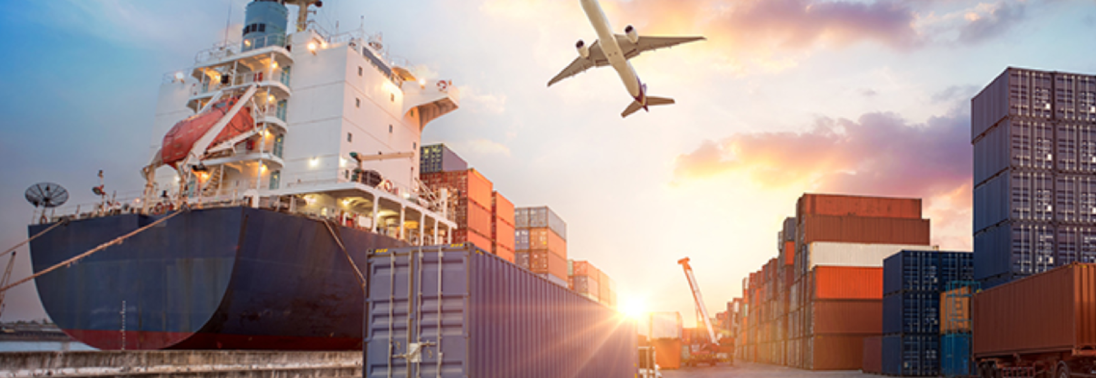
- Use the app higher up in the chapter if you like. Tip: think Y = AD = C + I + G + EXPORT − IMPORT. Then plug in everything you know and solve for GDP. For example: Y = AD = 100 + 0.8[Y − (10 + 0.4Y) + 80] + 50 + 80 + 20 − 20. Be careful with minus signs. I had ChatGPT compute Y = 550 (see here). Actual GDP is therefore 50 above potential, i.e. a 10% gap. Once Y = 550 you can compute government revenues (taxes) and compare to spending (government consumption + transfers). The budget deficit is 70, about 12.7% of GDP.
- This is exactly the same type of problem as above; the only difference is that imports here depend on GDP. First compute that GDP equals 245. Then substitute Y = 245 into the import function. If unsure, play with the app. Think: Y = AD = C + I + G + EXP − IMP = 45 + 0.8[Y − T + Tr] + 30 + 40 + 50 − (30 + 0.1Y). Watch the minus signs in front of parentheses.
- Use the app higher in the chapter if you get stuck.
- Tip: explain your answer using the figures below. Panic and collapsing wealth likely reduce AD, which in the short run lowers GDP (from 1 to 2 in the left‑hand figure). Firms then want fewer employees; if wages are sticky this produces higher unemployment. The crisis also makes dealing with Sweden less attractive: demand for SEK likely falls (fewer people need kronor to buy things in Sweden) while the supply of kronor rises (more want to sell their kronor). The krona therefore depreciates versus the euro.
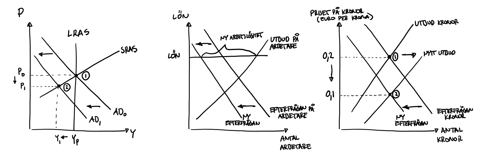
- Expansionary fiscal policy raises AD and thus Y, but in an open economy the increase is smaller. Why? Higher Y typically pushes up interest rates (booms increase borrowing demand). Higher rates strengthen the currency (attracting savings), and a stronger currency makes exports harder. So part of the stimulus is offset: G rises but EXPORT falls a bit. The net increase in AD (and thus Y) is therefore smaller than in a closed economy. For monetary policy the opposite holds: lower rates raise C and I and also weaken the currency, which boosts EXPORT.
- This last exercise is a tougher test but uses the exact same idea as before. Results: GDP ≈ 257.45; imports ≈ 78; taxes ≈ 35.75; transfers ≈ 17.13; deficit ≈ 1.38, about 0.5% of GDP.
- Heidi Schauman is Global Head of Research at Danske Bank. Previously she has served as chief economist at Swedbank and Aktia, and worked at Nordea and the Bank of Finland. I think she would make an excellent finance minister. Here is a guest lecture from autumn 2020 in which I interview her about her views on Finland and the world. Did Heidi’s predictions come true?