16 Unemployment
(where you learn why 297,000 Finns are out of work)
So far we have talked a lot about gross domestic product (GDP). Hopefully you now know quite a bit about the factors that determine how wealthy we become. Remember that the answer depends heavily on your time horizon. Use growth models to analyse the long‑run GDP level, but use the AD‑AS model to understand business‑cycle swings.
But sometimes GDP feels abstract — you may not care at all whether GDP rises or falls. So let us look at another part of the economy that may affect you more directly: the labour market. What will happen to you in working life? Will it be easy or hard to get a job? And what happens if you don’t get a job? That is the theme of this chapter.
16.1 The labour‑market situation?
Before we analyse how the labour market functions it is useful to know some key terms. In the figure below I have drawn one of the most common measures used in macroeconomics.
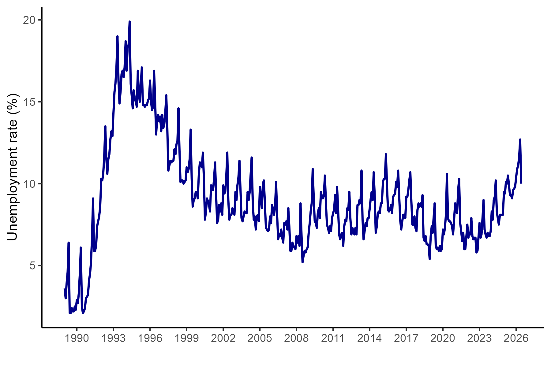
The figure above shows the unemployment rate, the number people usually mean when they talk about “unemployment”. What do you think when you see the chart? Perhaps that unemployment varies over time? At the end of the 1980s unemployment was 2 per cent, but a few years later it rose to as much as 20 per cent. Why did that happen? You might suspect Finland was hit by a recession — and that is indeed the case.
But another important insight from the figure is that unemployment is not driven only by the business cycle. Unemployment never falls to zero — so even in good times many Finns remain unemployed. Why is that?
To measure unemployment the authorities — in Finland’s case Statistics Finland — contact a random sample of adults and ask what they do during the day. They can then be classified into one of the following three groups:
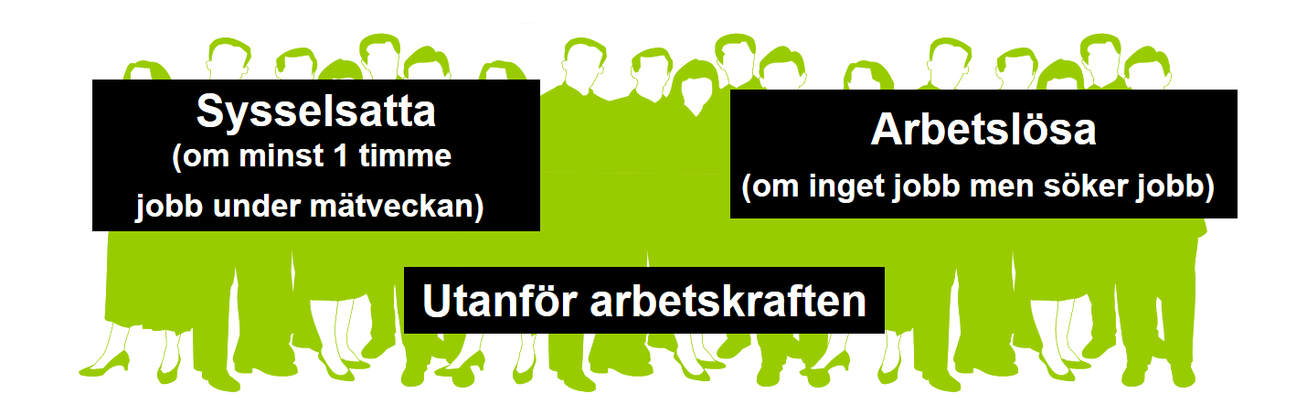
You are counted as employed if you worked at least one hour during the survey week. If you say you do not have a job but are actively looking for one, you are counted as unemployed. Together, the employed and the unemployed are called the labour force. The rest are outside the labour force — for example pensioners, students and people who feel it’s no longer worth looking for work. This is what the labour market looked like in June 2026 for people aged 15–74:
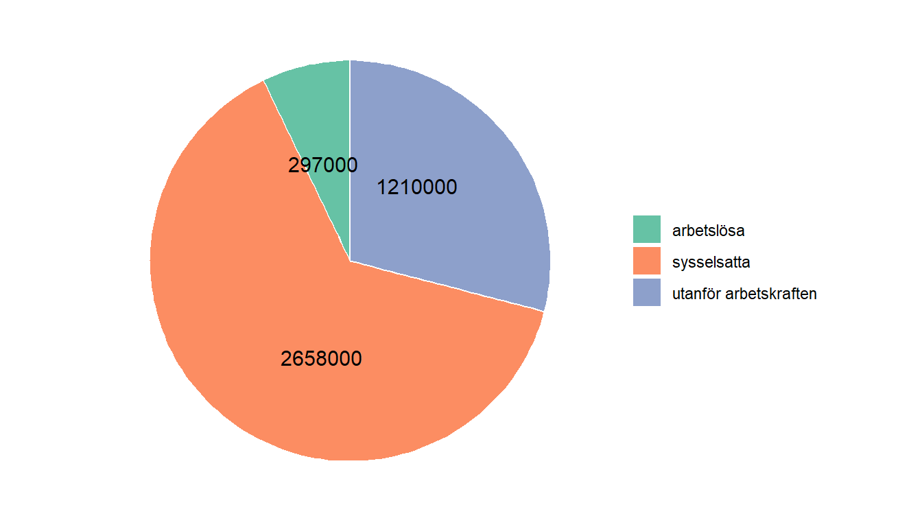
In June 2026 there were 2.658 million Finns aged 15–74 employed, 297 000 were unemployed and the remaining 1 210 000 were outside the labour force.
From these figures you can derive several measures of the labour‑market situation. The unemployment rate shows the share of unemployed as a percentage of the entire labour force (those who are either employed or unemployed). Right now the unemployment rate is about 10.05 per cent. You get this figure by dividing the number of unemployed by the sum of unemployed plus employed, and then multiplying the ratio by 100 to express it as a percentage.
Just as there are different variants of GDP, there are different measures to describe the labour market. An important metric is the employment rate, which shows the share of the working‑age population that is employed. In other words: what share of the circle in Figure 16.2 is orange? The answer is about 63,82 per cent. The labour‑force participation rate is a third common labour‑market measure. This shows the share of the adult population that is in the labour force. What share of the circle is therefore either orange or green? About 70,95 per cent.
the labour force consists of people who are either employed or unemployed
unemployed are people who do not have a job but are actively seeking work and ready to start; for example students and conscripts are not counted as unemployed because they are not in the labour force
the unemployment rate (or relative unemployment) is the share of unemployed within the labour force
hidden unemployment are working‑age people who do not work but have not registered as jobseekers despite being willing to take a job; causes include distrust in job prospects, childcare obligations or health reasons
the employment rate (or relative employment) shows the share of employed within a given population group
So why are so many people unemployed? If we don’t know the cause it’s hard to find a solution. In the next four sections we will therefore go through four different theories of why unemployment arises.
16.2 Frictional unemployment
In some ways we can liken the labour market to an outdoor café. Imagine the terrace at Domkyrkotorget, or better still the lively atmosphere on Piazza Navona in Rome on a warm summer evening.

The square is full of tables with hundreds of people dining, and there is always a lot of movement. Many people are looking for a free table, while other guests get up, pay and leave their seats.
Imagine there are currently 57 people on the square searching for a seat. You can think of them as unemployed. At the same time there are also 57 free seats, representing vacant jobs. It takes time for all 57 people to find their seats. The square is large and it’s hard to see where the free seats are. Even if you spot a table far away, it can take time to make your way between the tables.
Frictional unemployment is a type of unemployment. It arises, just like the queues on the square in Rome, because it takes time to match vacant seats with people who want a seat. When you graduate there may be a job that fits you perfectly, but it can still take weeks or months before you find each other.
So how can society improve matching to reduce frictional unemployment? Two factors seem crucial:
Improve information! Frictional unemployment often stems from lack of information. Your dream job may be in Kuopio, but you need to know about it to apply. An important task for organisations such as the employment office (TE‑office) is to help match jobseekers with employers who need to hire.
Strengthen the incentives to search for work! The figure below is from Carling et al. (2001), which follows thousands of people who became unemployed at a given point in time. The horizontal axis shows how many weeks have passed since they became unemployed, while the vertical axis shows the share of the group that found a job in each week. Half of the group received unemployment insurance (A‑kassa) and the other half did not. The benefit was paid only for 14 weeks and then stopped entirely.
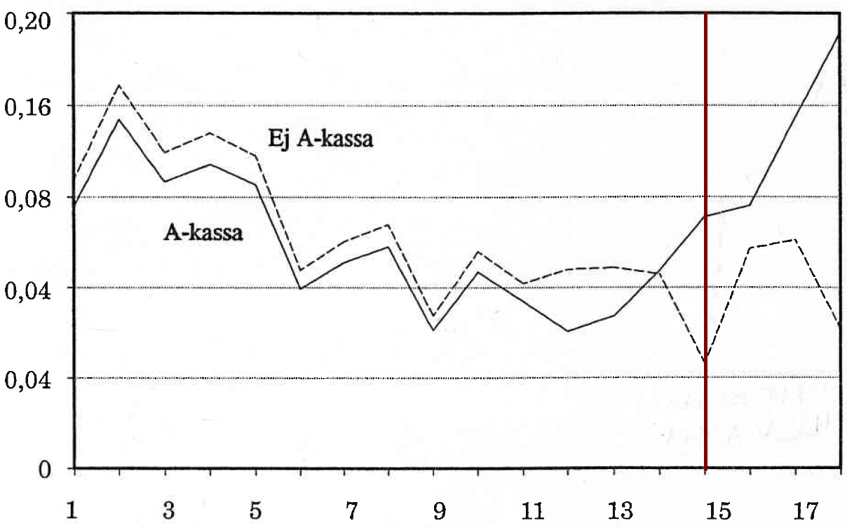
How should we interpret this figure? We see that about 8 per cent find a job already in the first week. In the following weeks progressively fewer find work. But after 14 weeks something interesting happens: the solid line suddenly jumps sharply. That group starts finding jobs! The odd thing is that this occurs exactly when their benefit ends. The same jump in job‑finding probability is not seen in the control group that never received benefits — so the phenomenon is unlikely to be due to something else that happened in society that week making jobs easier to get.
A similar study in Finland, Uusitalo & Verho (2010), showed that an increase in unemployment benefits in 2003 — from 52 to 60 per cent of previous wages — raised the duration of unemployment by 30 days. Do you remember Pontus in Chapter 1? He examined exactly this question in his bachelor thesis and found similar results.
Studies like these are sometimes used to justify cuts in benefit systems. But let’s think one step further! Imagine you graduate and immediately become unemployed and the unemployment benefit is €0. Or worse: for every day you are unemployed you are fined €1,000. That measure would surely make you take a job faster. But is it sensible policy? Maybe you are an economist, a lawyer or a surgeon — and now you must accept any job that comes along. The economist might end up in healthcare, the lawyer running fiscal policy and the surgeon delivering post. Not great, right?
Just as it’s important to take time to find the right food on the square, it is also important not only to focus on getting a job as quickly as possible but to ensure the job actually fits you.
16.3 Structural unemployment
Structural unemployment arises when the unemployed lack the skills firms need. This type of unemployment becomes more common when society changes rapidly.
In the 1980s, when I grew up in northern Sweden, things were simple. Most parents had similar educations, usually in industry or healthcare, and local employment was dominated by the hospital and the factory that made lawnmowers. It was probably easy to match parents to the available jobs. Those with technical training ended up at the factory and the rest found work at the hospital.


Today the world looks different. With new technology and globalisation societies change rapidly. New industries emerge and others disappear. You can now choose from thousands of specialised courses. All this drives the technological progress that, according to growth theories, is the route to sustained prosperity — but it also likely increases structural unemployment. The faster society changes, the more likely it is that the unemployed lack the skills firms need.
Before the Industrial Revolution in 18th‑century England few social changes occurred; it is said tools changed more slowly than the human skeleton. Then suddenly new technology broke through — and what firms needed was no longer what workers could offer. Protests against the new technology therefore turned violent. Here are a few lines about what happened when James Hargreaves invented the Spinning Jenny, a revolutionary machine that helped make England rich. Suddenly one worker could produce as much yarn as 200 workers had previously.
“The development of the machine led to protests and attacks by hand‑spinners who felt their future was threatened. Some spinners stormed James’s house and destroyed the Spinning Jenny, but he simply moved to another town and soon ‘Jenny’ existed in 20,000 improved copies. His neighbours feared the new machine and believed they would all become unemployed. In 1768 they formed a mob that ransacked Hargreaves’s home and destroyed his Jenny. Understandably upset, Hargreaves and his family moved to Nottingham. There he entered a partnership with Thomas James, and the two men opened their own cotton‑spinning mill.”
History is full of failed attempts to stop new technology and smarter ways of working. In the 1970s discos took off, which was the death knell for many dance bands. Click the image for a modern example of structural unemployment.
Today we see how artificial intelligence (AI) is rapidly changing our lives. As with earlier technological shifts, AI can create unemployment and protests. In summer 2023 actors in Hollywood went on strike to prevent AI from replacing them. Many people are worried. You may have read alarmist reports claiming half of jobs could be automated within 20 years. But new technology also creates new jobs. Historically roughly 10 per cent of jobs disappear and 10 per cent are created each year. Although technology can cause short‑term job losses, it also offers opportunities for new and better jobs in the long run. This is the creative destruction that growth theory says drives development when new firms replace old ones. The big change now is simply the speed at which this structural transformation occurs.
16.4 Classical unemployment
The third explanation for unemployment is that wages can become so high that firms do not want to hire as many workers as want to work. An example is when authorities introduce a minimum wage, which we discussed in Chapter 5. The figure below shows a simple model of the labour market for course assistants at Åbo Akademi.
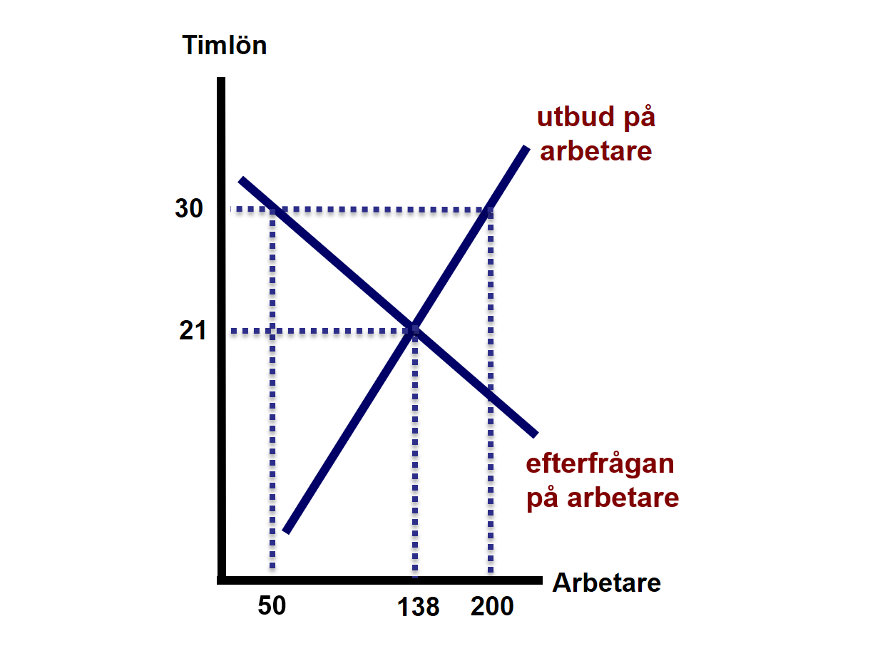
The vertical axis shows the hourly wage and the horizontal axis the number of workers. The supply curve shows how many students want to work as course assistants at different wages. If the hourly wage is €21, 138 ÅA students sign up; if the wage rises to €30, 200 want the job. The demand curve shows how many course assistants all departments at Åbo Akademi want to hire at different wages. The curve slopes downwards, which means the university wants to hire more when the wage is low.
On a free market the equilibrium wage would be €21 and 138 students would get jobs. In reality wages are often higher. Suppose the wage is €30. Here 200 students want to work as assistants, but only 50 get jobs. The remaining 150 become unemployed. This is called classical unemployment. But who is to blame for the wage ending up above the equilibrium? There are three suspects:
The students themselves! You students can organise to bargain for higher wages. Through a union you can raise the wage from €21 to €30. That’s great news for the 50 who get jobs at the higher pay, but it also increases unemployment. You may remember Tom Joad and his search for work in 1930s America? President Hoover and economists of the time thought high unemployment was precisely due to workers demanding excessive wages.
The employers! Why would Åbo Akademi voluntarily pay course assistants like Julen and Sami more than the market wage? To understand this we go back to the USA in 1914. Henry Ford, one of America’s richest and most admired men, introduced the assembly line — but he also did something else decisive: he sharply raised wages from USD 2.25 a day to USD 5 a day. Immediately hordes of jobseekers gathered outside the factory. Suddenly everyone wanted to work for Ford. At the same time employee productivity rose. Maybe they wanted to repay Ford’s generosity? Maybe they were motivated by the long queue outside? Whatever the reason, the result was clear: no one loafed any more, everyone turned up on time and work quality improved. This is called the efficiency‑wage theory. Raising wages — contrary to intuition — increased Ford’s profits. Similarly, a high wage for course assistants can benefit Åbo Akademi because those hired will work hard. The downside is that it also creates unemployment.
The politicians! In a free market wages are set by supply and demand, but politicians sometimes intervene to influence wages. For example, they can introduce statutory minimum wages for course assistants. The effect can again be higher wages for those employed, but also higher unemployment.
frictional unemployment is temporary unemployment that arises during life transitions, such as moving or after finishing studies
cyclical unemployment rises in downturns when firms lay off workers because demand falls and then falls again when the cycle turns up
matching problems occur when unemployed workers and vacancies do not match each other due to, for example, skill gaps or geographic distance
structural unemployment arises from structural changes in the economy, such as technological progress or globalisation
16.5 Cyclical unemployment
So far we have covered three types of unemployment: frictional, structural and classical. All of these exist even when the GDP gap is zero. We therefore often call this unemployment the natural rate — the level of unemployment we can expect in the long run.
But there is another reason people become unemployed: the business cycle. Cyclical unemployment (also called demand‑deficiency unemployment) causes unemployment to rise in recessions and fall in booms. You can imagine demand for course assistants falling when Finland’s economy weakens and the university is forced to cut back. In Figure 16.3 this means the demand curve shifts left. If the wage is stuck at €30, the number of unemployed will increase. In booms the demand curve shifts right and unemployment falls.
So what actually happens to unemployment when the economy deteriorates? As usual in economics you can analyse the data to see how the world behaves. I therefore downloaded data on unemployment and economic growth in Finland for 1991–2019 and plot the relationship in the following figure:
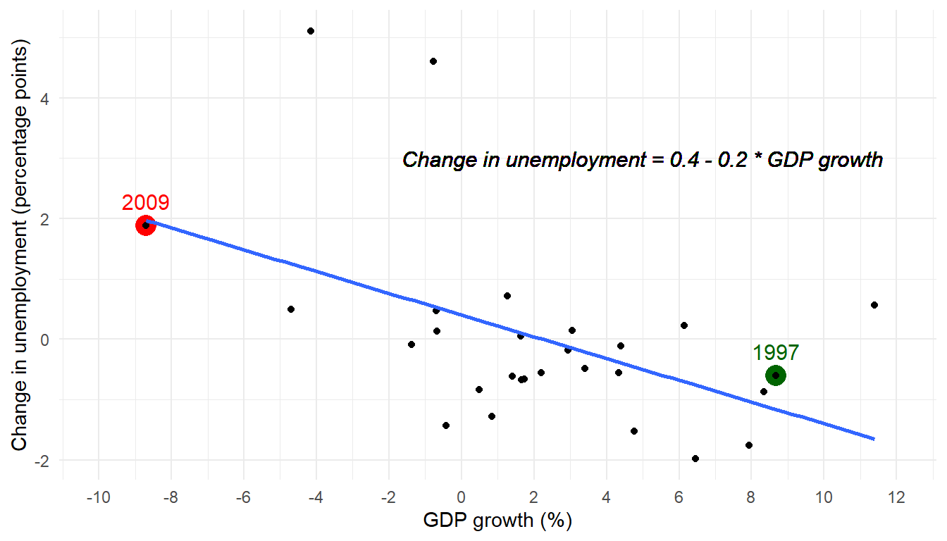
The horizontal axis shows economic growth and the vertical axis shows how unemployment has changed year‑on‑year. Each dot is Finland in a particular year. For example, the red dot at the far left shows 2009: GDP fell by 8.7 per cent and unemployment rose by 1.9 percentage points. The green dot near the far right shows 1997, when GDP grew by 8.7 per cent and unemployment fell by 0.6 percentage points (from 15.6% to 15.0%).
Remember the difference between percent and percentage points. If the share of students majoring in economics rises from 10 per cent to 15 per cent, that is an increase of 5 percentage points, which is a 50 per cent increase in relative terms.
I had the computer draw the best‑fit line summarising the relationship between the two variables. The line slopes downwards, meaning high growth tends to lower unemployment and vice versa. The computer also prints the line’s equation. This relationship between economic growth and unemployment is called Okun’s law. You can use Okun’s law to forecast how high unemployment will be in Finland.
For example, if you expect GDP to grow by 8 per cent in 2026, unemployment is forecast to fall by 1.2 percentage points (that is, 0.4 − 0.2 × 8). If instead you expect GDP to shrink by 5 per cent, Okun’s law predicts unemployment will rise by 1.4 percentage points.
How does unemployment respond to economic growth?
It’s straightforward to estimate Okun’s law for several countries and see whether the relationship differs across them. Let’s, for example, plot the relationships for Sweden, the USA and Japan for the period 1991–2019.
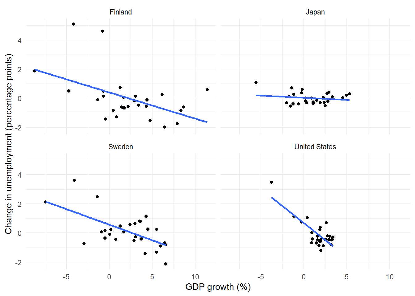
The four charts above show Okun’s law for Finland, Sweden, Japan and the USA for 1991–2019. As you can see, there are clear cross‑country differences. In Japan unemployment hardly responds to changes in growth — the Japanese therefore need not worry much about losing jobs when growth slows, but unemployment also doesn’t fall much in good times. In the USA the relationship is much stronger: low growth, typical of recessions, leads to sharply higher unemployment. In Sweden growth appears to affect unemployment roughly similarly to Finland.
16.6 The consequences of unemployment
Unemployment has large costs, both for individuals and for society.
Economic costs
Being unemployed leads to lower incomes for the affected person — even in the long run. What do you make of the following research findings?
- Finns who became unemployed during the 1990s crisis still have lower incomes than comparable people who did not become unemployed.
- People who were unemployed immediately after upper secondary school have, five years later, annual incomes 17 per cent lower than their siblings who did not become unemployed straight after school.
- Unemployment appears to erode skills. Edin & Gustavsson (2008) analyses results from a large Swedish skills test. Some participants lost their jobs afterwards. A few years later everyone took the same test again. The unemployed performed substantially worse the second time, while those who had been continuously employed showed no decline in test scores.
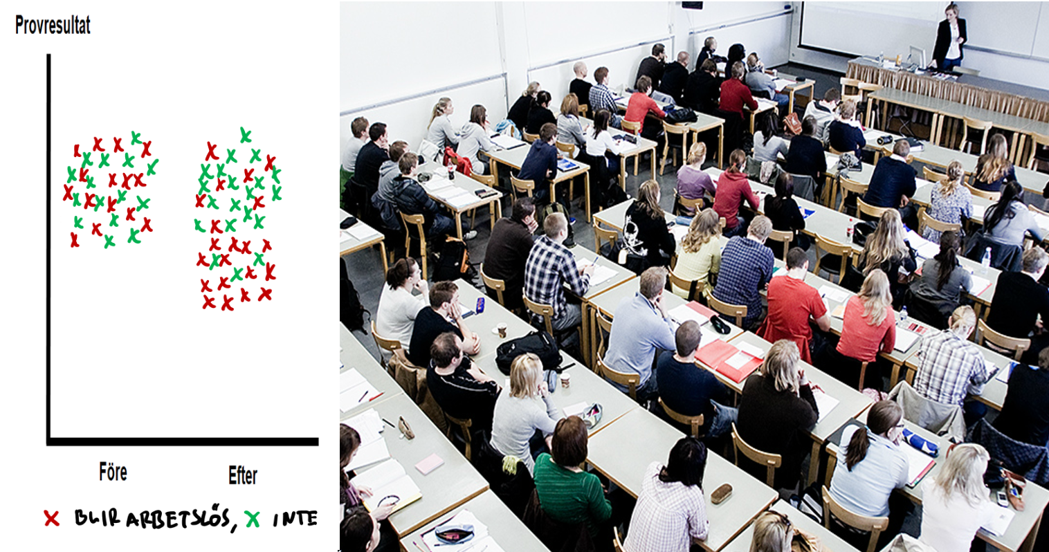
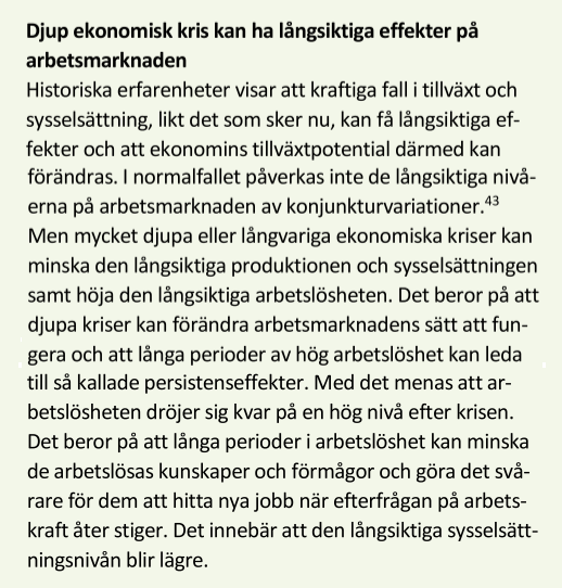
It’s not only during the unemployment spell that you suffer financially. The effect can persist long afterwards. It therefore seems that a temporary rise in unemployment — for example due to a pandemic — can also cause permanent damage to the economy. A temporary downturn leaves scars that never fully heal. This phenomenon is called hysteresis. You can think of time spent unemployed as eroding your skills: parts of what you once knew fade away. When you finally find work again you are not quite the same person as before. It is as if the LRAS curve has shifted slightly to the left.
Does a temporary crisis cause permanent damage?
As always in economics, you can go out and measure the relationship in the real world. Let us therefore investigate whether there is evidence that hysteresis exists in Finland. For example, did the 2007–2010 financial crisis leave a lasting mark on Finland’s labour market? To examine this I downloaded quarterly data from Statistics Finland on unemployment and job vacancies from 2001 onward. In the figures below I plotted the relationships:
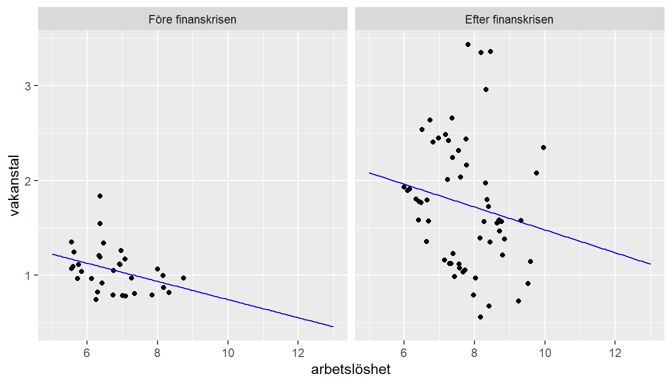
The left‑hand chart shows the labour‑market situation during 2001–2008 and the right‑hand chart shows the corresponding situation after the financial crisis. Each dot is a quarter. The horizontal axis shows unemployment and the vertical axis shows the so‑called vacancy rate. The vacancy rate measures the number of vacancies relative to the size of the labour force (as a percentage). For example, if there are 100 people in the labour force and 5 vacancies, the vacancy rate is 5.
In both charts there is a fairly clear negative relationship between vacancies and unemployment: when there are many vacancies unemployment is usually low, and when there are few vacancies many are unemployed. This negative relationship is called the Beveridge curve, illustrated by the blue lines in the figure.
But there is also an interesting difference between the panels. Isn’t the Beveridge curve much further to the right after the financial crisis? Look, for example, at the vacancy rate of 1. When there were that many vacancies in the first half of the 2000s unemployment according to the Beveridge curve was about 7 per cent, but after the financial crisis unemployment was over 13 per cent at the same vacancy rate. What can explain this? Perhaps it is an effect of what happened in Finland during the crisis. Maybe Finns lost part of their human capital that is so important for technological development. This also worsens matching on the labour market: there are as many jobs as before but we have become “worse” at filling them, so it takes longer to match vacancies with jobseekers. The result is high unemployment even when vacancies are plentiful. If you believe a temporary crisis can leave long‑term traces, you have an additional argument for fighting downturns with expansionary policy.
Exercises
In this chapter you have learned more about the causes and consequences of unemployment. Press Show Answers when you want the computer to grade your responses. Good luck!
Can early retirement eliminate unemployment?
In 2016 you are the economic adviser to the leading opposition politician in the country. Her campaign promise is to bring unemployment below 5 per cent. The table below shows what Finland’s labour market looked like during 2009–2016. I’m sorry that information in some cells is missing.
| Year | Employed | Unemployed | Persons of working age (15–74) | Employment rate (%) | Unemployment rate (%) |
|---|---|---|---|---|---|
| 2009 | 2,457,000 | 221,000 | 4,025,000 | 61.1 | 8.25 |
| 2010 | 2,447,000 | 224,000 | 4,043,000 | 60.5 | |
| 2011 | 2,474,000 | 209,000 | 4,059,000 | 7.79 | |
| 2012 | 2,483,000 | 4,075,000 | 60.9 | 7.70 | |
| 2013 | 2,457,000 | 219,000 | 4,087,000 | 60.1 | 8.18 |
| 2014 | 2,447,000 | 232,000 | 59.8 | 8.69 | |
| 2015 | 252,000 | 4,102,000 | 59.4 | 9.37 | |
| 2016 | 2,448,000 | 237,000 | 4,109,000 | 59.6 | 8.82 |
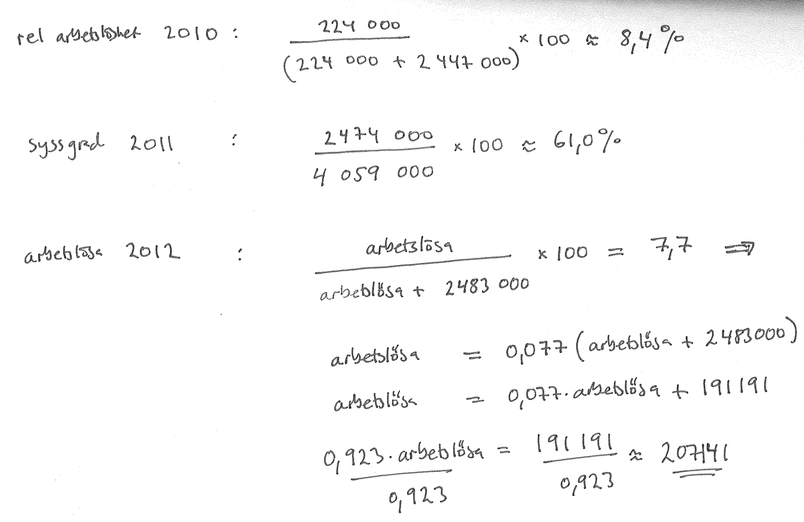
- Your boss wants you to immediately fill in the missing cells, which is possible if you know how the different measures are calculated: the unemployment rate in 2010 was ; the employment rate in 2011 was ; the number of unemployed in 2012 was approximately ; the working‑age population (15–74) in 2014 was approximately ; and the number employed in 2015 was approximately .
- We have reviewed four different theories explaining why a person is unemployed. Each theory also suggests a policy to fight unemployment. Give a concrete political proposal for how to combat each type of unemployment. Express yourself simply so everyone understands.
- To help your boss meet her election pledge you recommend that at the end of 2016 she puts half of all unemployed people onto early retirement. What happens? The pledge because the unemployment rate (to two decimal places) becomes: .
- Also enter how the reform affects the other measures. The employment rate becomes and the labour‑force participation rate becomes .
- Start from the formulas in Section 16.1. For some subquestions you must be a bit clever: in one question you know the unemployment rate and the number employed, but not the number unemployed. One way is to trial the answer choices, but a smarter way is to solve the problems analytically as shown below.
- Review frictional, structural, classical and cyclical unemployment. Then write a well‑worked answer proposal. Read your answer aloud to yourself — can you be understood? Practice expressing yourself clearly.
- Think about what this implies: you can reduce the unemployment rate by, for example, putting people on early retirement or forcing them into pointless training. The Swedish government promised in the late 1990s to “bring unemployment below 4 percent”. The pledge was met, but critics argued it happened mainly through early retirements and training programmes.
- It is therefore often useful to look at alternative measures, such as the employment rate and labour‑force participation. Note that early retirement reduces the unemployment rate, leaves the employment rate unchanged and lowers the participation rate.
Causes of unemployment
Unemployment in Finland is currently unusually high. On YLE newly graduated Emmy testifies how she had to send hundreds of applications before she finally got a break.
- In this chapter we covered four explanations for why unemployment occurs. What are these four types of unemployment, and what does each theory say is the reason people become unemployed?
- You are now appointed Minister for Labour. Congratulations! Your task is to reduce youth unemployment in Finland. How would you do it — and what are the drawbacks of your proposals?
- What does Okun’s law state?
- What does the Beveridge curve show?
- What does the term hysteresis mean?
- When crime fell sharply in the US in the early 1990s many experts argued the main cause was the strong economy — low unemployment typically reduces crime. Steven Levitt, however, argued the main explanation was something entirely different. According to Levitt, what was the largest explanation for the crime decline?
- Review frictional, structural, classical and cyclical unemployment. NOW try writing your answer on paper. Many students think they can answer a question but discover during the exam that they cannot. Read your answer aloud — is it clear and understandable?
- Base your response on the four types of unemployment. What policy does each theory suggest — and why might that be problematic? Example: frictional unemployment suggests shortening benefit durations to reduce unemployment spells, but cutting benefits for already vulnerable groups can be ethically and politically problematic.
- Read the chapter and prepare a good answer.
- Read the chapter and prepare a good answer.
- Read the chapter and prepare a good answer.
- Watch Levitt’s video — it’s interesting!
The crisis hits in 1990
In the early 1990s Finland was suddenly thrown into its deepest economic crisis in modern times. The figure below shows unemployment rising from 3.2 per cent in 1990 to almost 17 per cent in the following years.
- Unemployment varies sharply by age group, by gender and by month. Think of your grandmother and how old she was in November 1993. What was the unemployment rate (the relative unemployment rate) for women in your grandmother’s age group? You can find the data here.
- Hysteresis means a temporary downturn causes permanent damage to the economy. In our AD‑AS model this can be illustrated as a leftward shift of the LRAS. Name one plausible reason why the 1990s crisis might have harmed Finland’s ability to produce goods and services even in the long run.
- In the chapter I plotted the Beveridge curve for the period before and after the 2008 financial crisis. Suppose you do the same exercise for the period before and after the 1990s crisis and find the Beveridge curve has shifted to the right. What conclusions would you draw from that pattern?
- Note how extraordinarily high unemployment was in Finland during the 1990s crisis.
- A leftward shift of LRAS means potential GDP falls. Likely the natural rate of unemployment rises as well. To understand the change in our long‑run welfare level look to growth theory: how could the temporary 1990s crisis have reduced labour, capital or technology? For example, did people suffer permanent scarring, lose human capital, become worse at job search, or lose their ability to innovate?
- A rightward shift of the Beveridge curve implies that for a given number of vacancies unemployment is now higher than before. A plausible explanation is worsened matching (higher frictional unemployment): it takes longer to match vacancies with jobseekers, perhaps because time spent unemployed has eroded skills.
Social costs
Unemployment is not limited to euros and cents. The social costs are large. Many studies have examined how people are affected by job loss. The unemployed fare worse than other groups. Unemployment affects the children in the family. Higher unemployment also raises certain types of crime. Studies in the economics of crime show that a 1 per cent increase in unemployment leads to roughly 1.5 per cent more burglaries. The effect on violent crime is, however, disputed. Unfortunately, the list of social costs can be made long.
In the early 1990s crime in the United States suddenly fell like a stone, contrary to what almost all criminologists had predicted. But why did crime fall? Many argued afterwards that it must have been due to the strong economy; low unemployment usually leads to fewer crimes. But there are many alternative explanations. Some say it was tougher policing methods that reduced crime. Was it stricter gun laws? Or falling crack prices that made crime less profitable? Economist Steven Levitt, known for the readable book Freakonomics, argues in the following clip that the answer is something entirely different. His controversial results provoked an enormous debate in the US: